Wrangling and Visualizing Historical Texts
By Laurie Baker
Acknowledgements

Slide Structure and Design inspired by Julia Silge
What can you do with R? A snapshot
Influence of target species on fishing effort

Who is fishing?
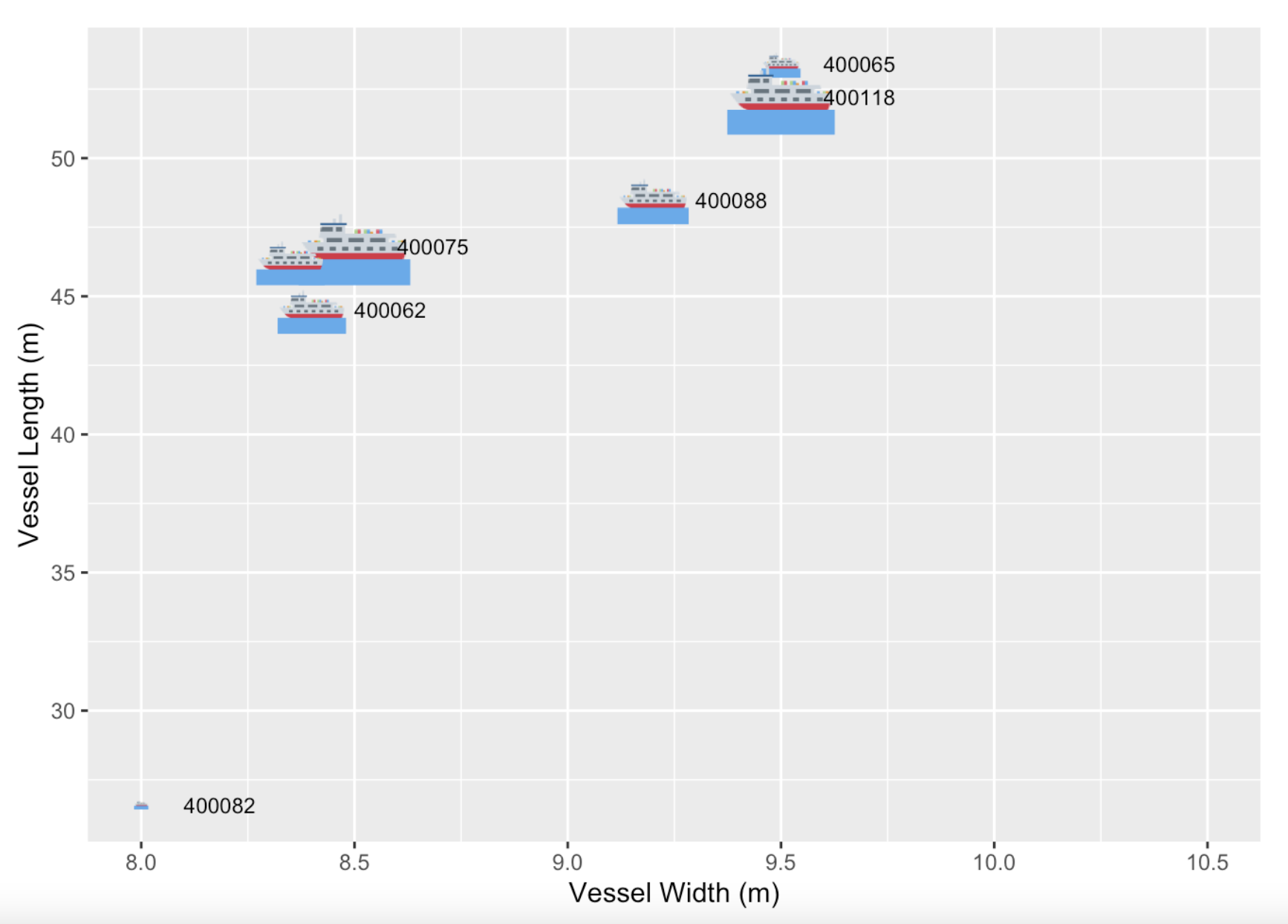
How are vessels fishing?
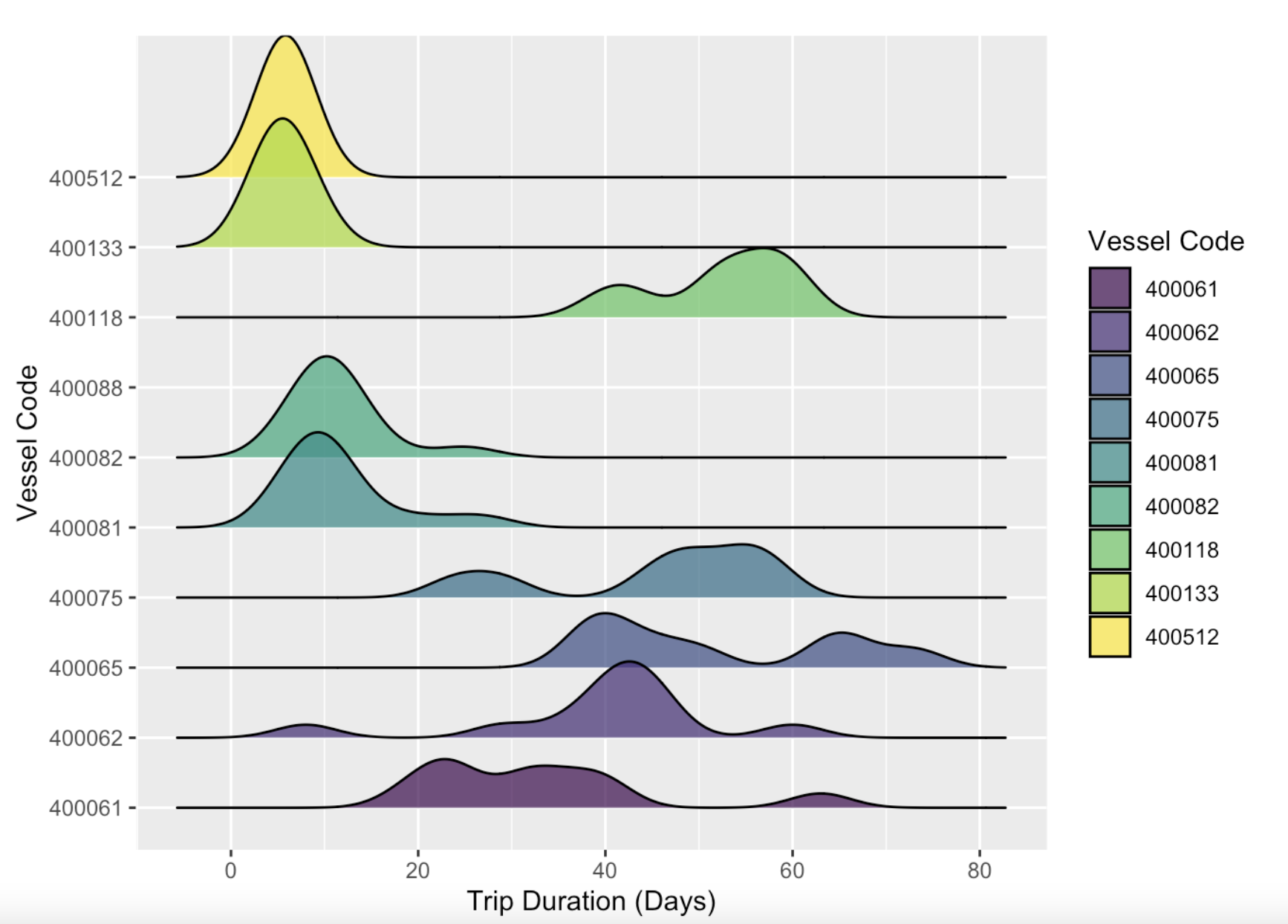
What are vessels targeting?
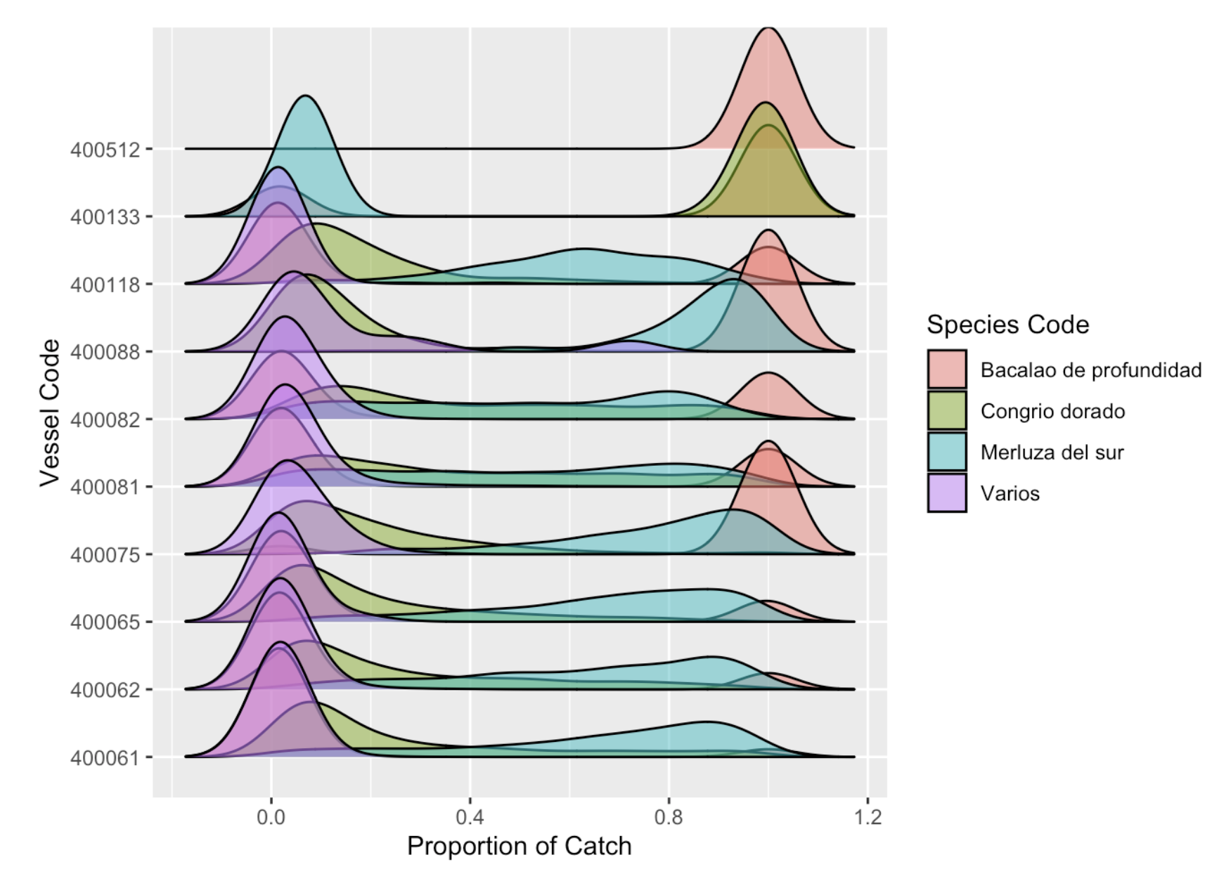
Where are they fishing?
What else can R do?
Create open source learning resources
Code Mitten Patterns
Choose colors for mitten patterns
Monitor fish runs
Build websites!
Goals for this week
- Get you coding and exploring text data.
- Help you see ways you could use R in your projects.
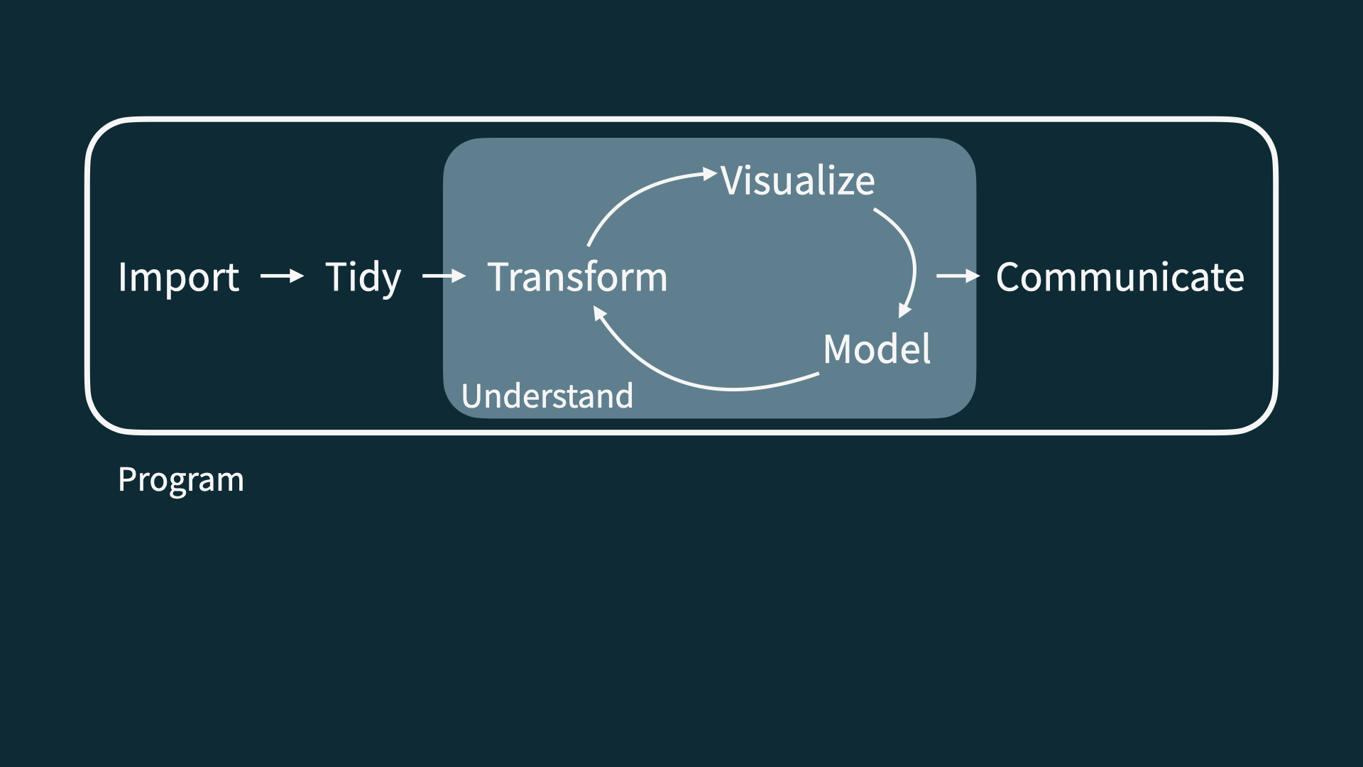
Data Science Life Cycle
Data Science Life Cycle
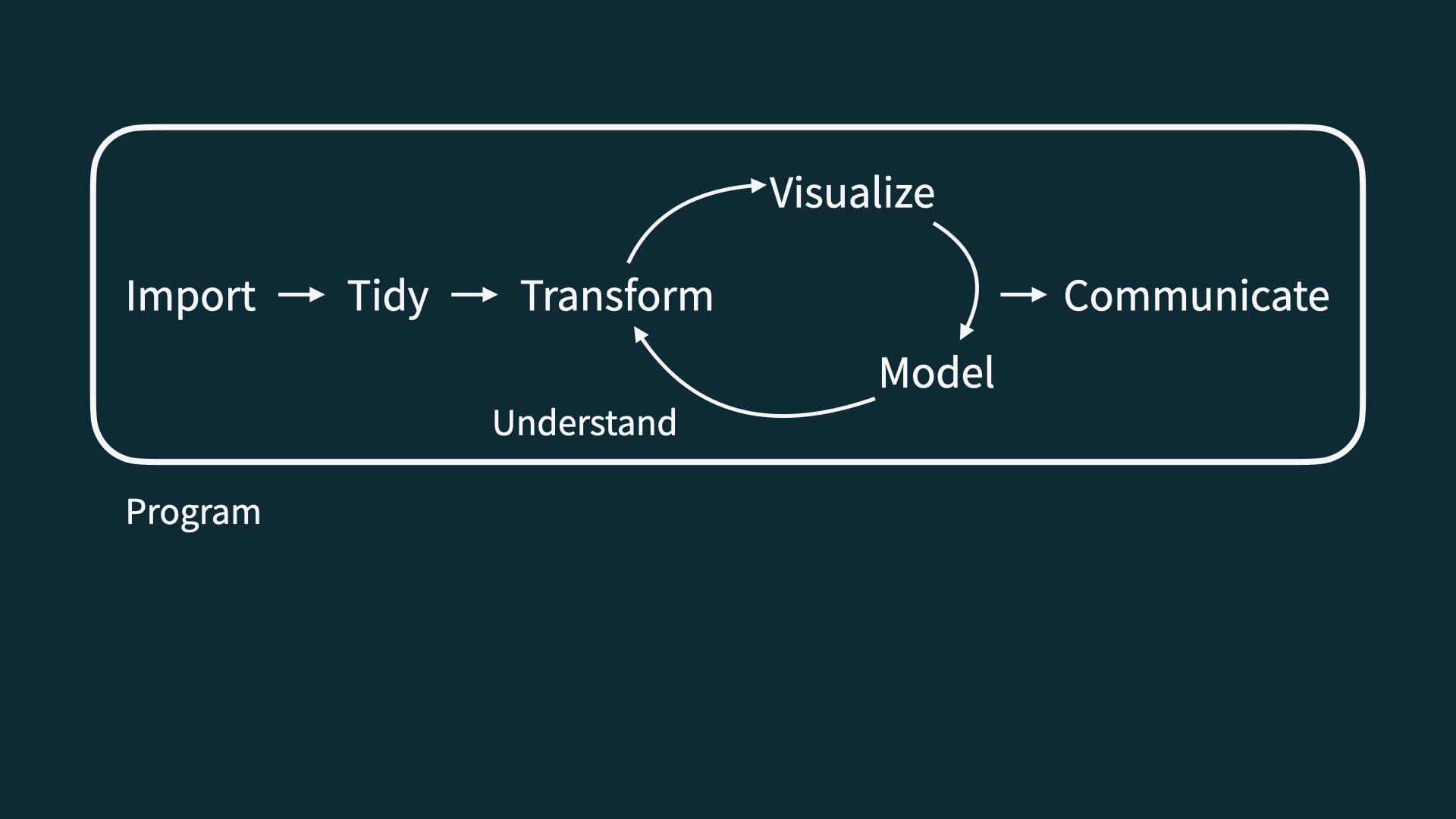
Data Science Life Cycle
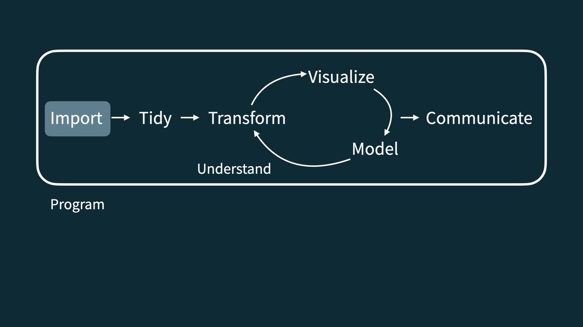
Data Science Life Cycle
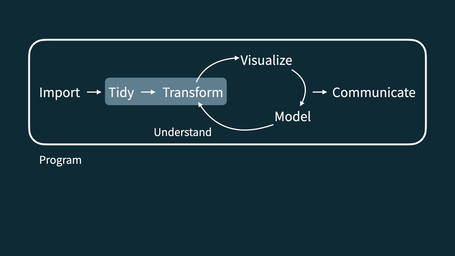
Data Science Life Cycle
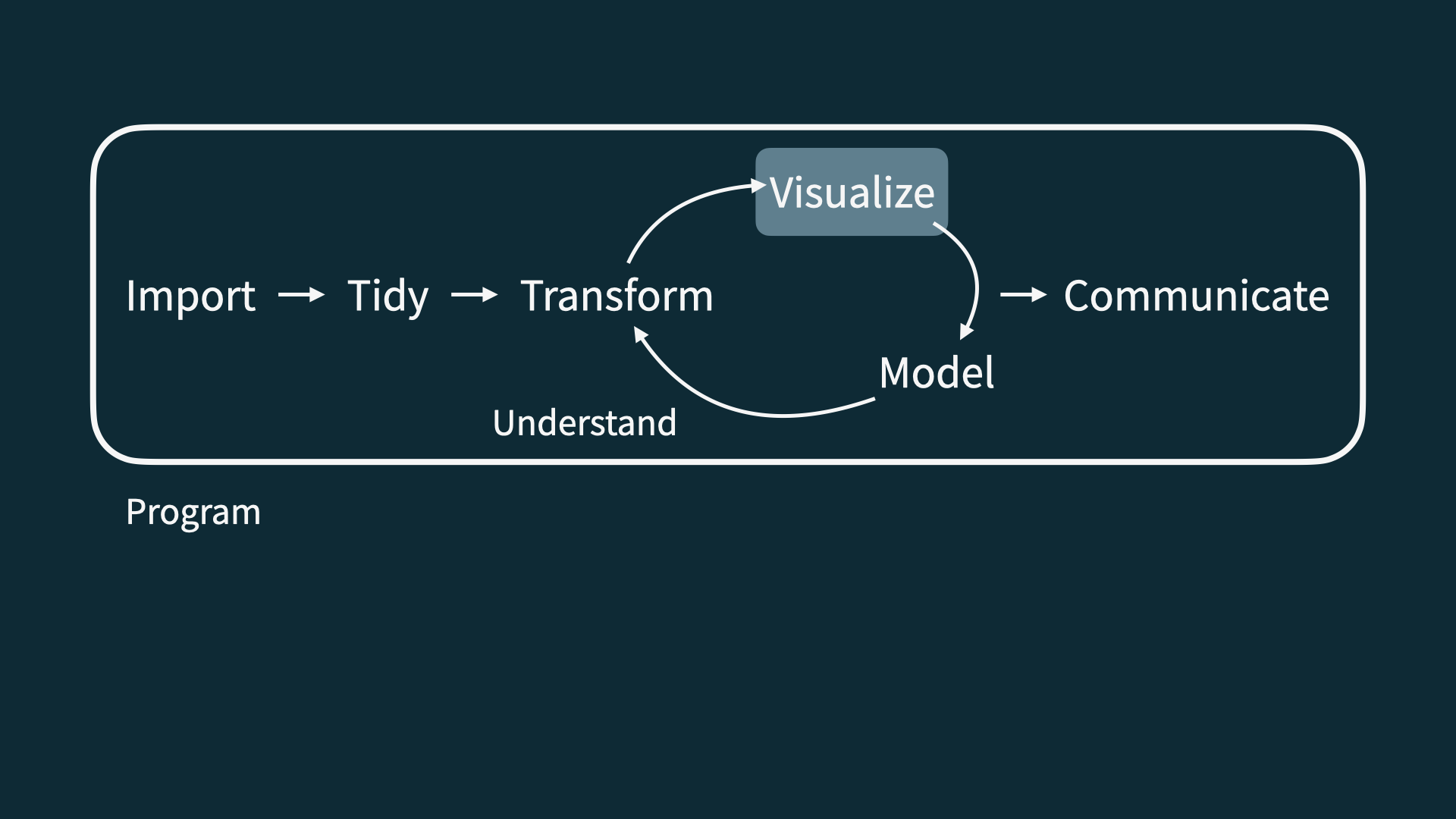
Data Science Life Cycle
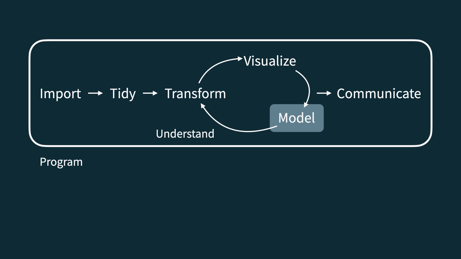
Data Science Life Cycle
Learning Objectives:
Learn how to
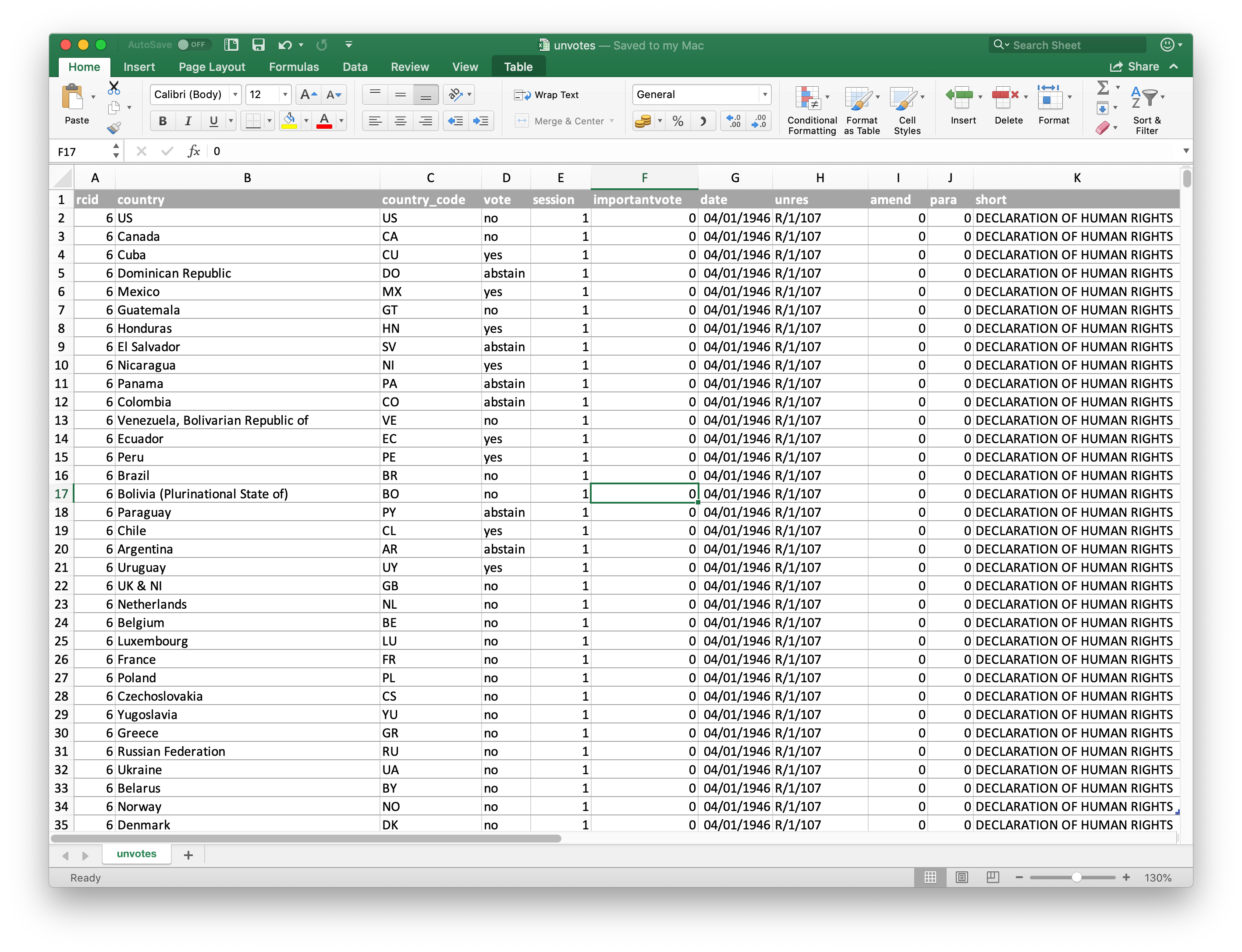
- Read in data using
read_excel - Select columns using
select - Create new variables using
mutate - Summarize and arrange data using
countandarrange - Group data to display and calculate multiple things
- Correct entries using
mutateandcase_when - Visualize and map changes in space and time using
ggplotandleaflet
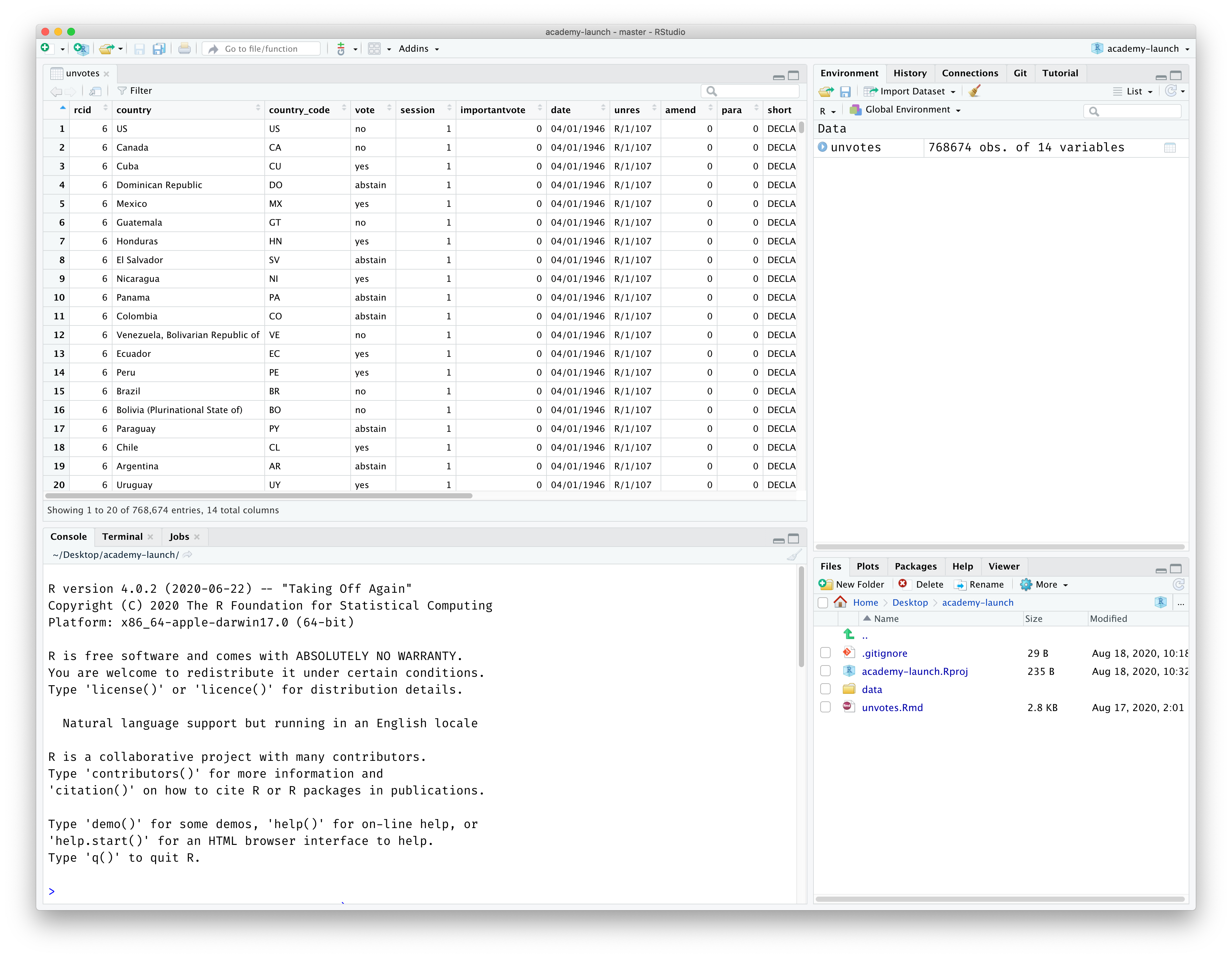
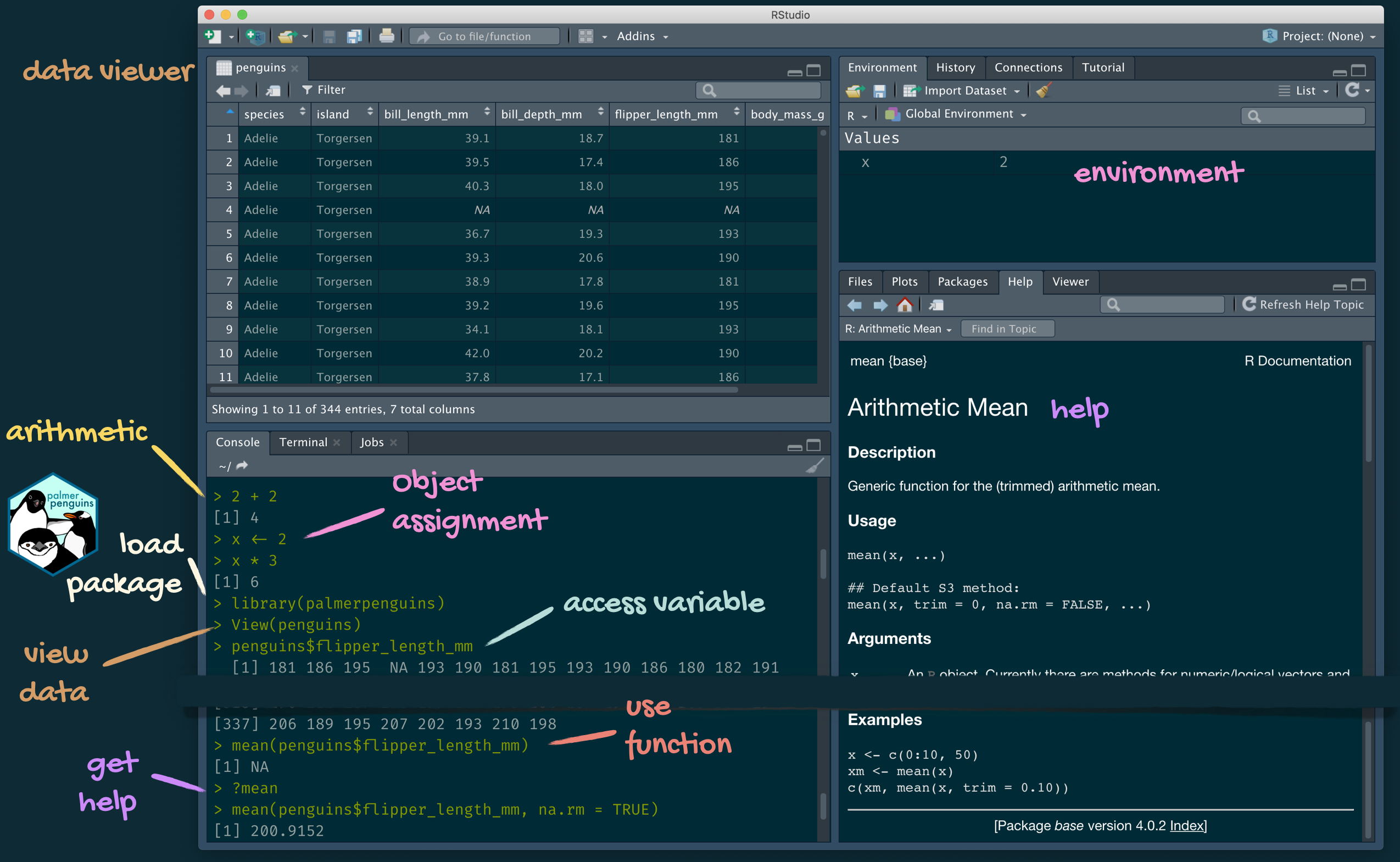
Introducing Posit Cloud

Let’s install some packages
- What are packages? You can think of them like toolboxes with different sets of tools (i.e.
functions) we can apply to our data
The Journals (1870-1906)
12 journals (1871-1883) transcribed
library(readxl)
journal_1871_1872 <- read_excel("data/journal_1871_1872.xlsx")
journal_1873 <- read_excel("data/journal_1873.xlsx")
journal_1874 <- read_excel("data/journal_1874.xlsx")
journal_1875 <- read_excel("data/journal_1875.xlsx")
journal_1876 <- read_excel("data/journal_1876.xlsx")
journal_1877 <- read_excel("data/journal_1877.xlsx")
journal_1878 <- read_excel("data/journal_1878.xlsx")
journal_1879 <- read_excel("data/journal_1879.xlsx")
journal_1880 <- read_excel("data/journal_1880.xlsx")
journal_1881 <- read_excel("data/journal_1881.xlsx")
journal_1882 <- read_excel("data/journal_1882.xlsx")
journal_1883 <- read_excel("data/journal_1883.xlsx")
Keeping Track
library(tidyverse)

journal_1871_1872$journal <- 1
journal_1873$journal <- 2
journal_1874$journal <- 3
journal_1875$journal <- 4
journal_1876$journal <- 5
journal_1877$journal <- 6
journal_1878$journal <- 7
journal_1879$journal <- 8
journal_1880$journal <- 9
journal_1881$journal <- 10
journal_1882$journal <- 11
journal_1883$journal <- 12

journals <- dplyr::bind_rows(journal_1871_1872, journal_1873, journal_1874,
                             journal_1875, journal_1876, journal_1877,
                             journal_1878, journal_1879, journal_1880,
                             journal_1881, journal_1882, journal_1883)
We have a lot of variables recorded!
glimpse(journals)
#> Rows: 5,509
#> Columns: 39
#> $ date_mdy                <chr> "12/23/1871", "12/24/1871", "12/25/1871", "12/…
#> $ month                   <chr> "December", "December", "December", "December"…
#> $ journal_entry           <chr> "Was married at home in evening by William Ran…
#> $ transcription           <chr> "confident", "confident", "confident", "confid…
#> $ location                <chr> "Winter Harbor", "NA", "Winter Harbor", "Winte…
#> $ location_accuracy       <chr> "mentioned", "NA", "assumed", "mentioned", "me…
#> $ local_place             <chr> "Home", "NA", "Hall", "Home", "Home", "Home", …
#> $ local_place_accuracy    <chr> "mentioned", "NA", "mentioned", "mentioned", "…
#> $ latitude                <chr> "NA", "NA", "NA", "NA", "NA", "NA", "NA", "NA"…
#> $ latitude_origin         <chr> "NA", "NA", "NA", "NA", "NA", "NA", "NA", "NA"…
#> $ longitude               <chr> "NA", "NA", "NA", "NA", "NA", "NA", "NA", "NA"…
#> $ longitude_origin        <chr> "NA", "NA", "NA", "NA", "NA", "NA", "NA", "NA"…
#> $ quantity                <chr> "NA", "NA", "NA", "NA", "NA", "NA", "NA", "NA"…
#> $ unit                    <chr> "NA", "NA", "NA", "NA", "NA", "NA", "NA", "NA"…
#> $ item                    <chr> "NA", "NA", "NA", "NA", "NA", "NA", "NA", "NA"…
#> $ letter                  <chr> "no letter", "no letter", "no letter", "no let…
#> $ letter_from             <chr> "NA", "NA", "NA", "NA", "N. H. Higgins", "NA",…
#> $ letter_to               <chr> "NA", "NA", "NA", "NA", "NA", "Na", "Na", "Na"…
#> $ wind_direction_am       <chr> "NA", "NA", "NA", "NA", "NA", "NA", "NA", "NA"…
#> $ wind_direction_pm       <chr> "NA", "NA", "NA", "NA", "NA", "NA", "NA", "NA"…
#> $ wind_direction_night    <chr> "NA", "NA", "NA", "NA", "NA", "NA", "NA", "NA"…
#> $ wind_speed_am           <chr> "NA", "NA", "NA", "NA", "NA", "NA", "NA", "NA"…
#> $ wind_speed_pm           <chr> "NA", "NA", "NA", "NA", "NA", "NA", "NA", "NA"…
#> $ wind_speed_night        <chr> "NA", "NA", "NA", "NA", "NA", "NA", "NA", "NA"…
#> $ weather_condition_am    <chr> "NA", "NA", "NA", "NA", "NA", "NA", "NA", "NA"…
#> $ weather_condition_pm    <chr> "NA", "NA", "NA", "NA", "NA", "NA", "NA", "NA"…
#> $ weather_condition_night <chr> "NA", "NA", "NA", "NA", "NA", "NA", "NA", "NA"…
#> $ temperature_am          <chr> "NA", "NA", "NA", "NA", "NA", "NA", "NA", "NA"…
#> $ temperature_pm          <chr> "NA", "NA", "NA", "NA", "NA", "NA", "NA", "NA"…
#> $ temperature_night       <dbl> NA, NA, NA, NA, NA, NA, NA, NA, NA, NA, NA, NA…
#> $ image_path              <chr> "NA", "NA", "NA", "NA", "NA", "NA", "NA", "NA"…
#> $ image_description       <chr> NA, NA, NA, NA, NA, NA, NA, NA, NA, NA, NA, NA…
#> $ recorder                <chr> "NH", "NH", "NH", "NH", "NH", "NH", "NH", "NH"…
#> $ notes                   <chr> "Esqr? Esquire", "to?", "Christmas tree?", NA,…
#> $ noteworthy              <chr> NA, NA, NA, NA, NA, NA, NA, NA, NA, NA, NA, NA…
#> $ second_check            <chr> "WD, EP", "EP", "WD, EP", "EP", "WD, EP", "EP"…
#> $ journal                 <dbl> 1, 1, 1, 1, 1, 1, 1, 1, 1, 1, 1, 1, 1, 1, 1, 1…
#> $ transcription_accuracy  <chr> NA, NA, NA, NA, NA, NA, NA, NA, NA, NA, NA, NA…
#> $ ...1                    <chr> NA, NA, NA, NA, NA, NA, NA, NA, NA, NA, NA, NA…
Exploring a subset using select
(journals_sub <- journals %>%
    select(date_mdy, journal_entry, location))
#> # A tibble: 5,509 × 3
#>    date_mdy   journal_entry                                             location
#>    <chr>      <chr>                                                     <chr>
#>  1 12/23/1871 Was married at home in evening by William Rand Esqr.      Winter …
#>  2 12/24/1871 Went to meeting.                                          NA
#>  3 12/25/1871 Shooting match all day in the evening to Christmas tree … Winter …
#>  4 12/26/1871 About home at work jobbing.                               Winter …
#>  5 12/27/1871 Work about home reed letter from N. H. Higgins Ins agt.   Winter …
#>  6 12/28/1871 Work about home.                                          Winter …
#>  7 12/29/1871 To work in shop.                                          Winter …
#>  8 12/30/1871 To work in shop.                                          Winter …
#>  9 12/31/1871 Went to meeting.                                          Winter …
#> 10 1/1/1872   Work in shop.                                             Winter …
#> # ℹ 5,499 more rows
Creating new variables using mutate
library(lubridate)
(journals_sub <- journals_sub %>%
    mutate(date_mdy = mdy(date_mdy),
           year = year(date_mdy),
           month = month(date_mdy)))
#> # A tibble: 5,509 × 5
#>    date_mdy   journal_entry                                 location  year month
#>    <date>     <chr>                                         <chr>    <dbl> <dbl>
#>  1 1871-12-23 Was married at home in evening by William Ra… Winter …  1871    12
#>  2 1871-12-24 Went to meeting.                              NA        1871    12
#>  3 1871-12-25 Shooting match all day in the evening to Chr… Winter …  1871    12
#>  4 1871-12-26 About home at work jobbing.                   Winter …  1871    12
#>  5 1871-12-27 Work about home reed letter from N. H. Higgi… Winter …  1871    12
#>  6 1871-12-28 Work about home.                              Winter …  1871    12
#>  7 1871-12-29 To work in shop.                              Winter …  1871    12
#>  8 1871-12-30 To work in shop.                              Winter …  1871    12
#>  9 1871-12-31 Went to meeting.                              Winter …  1871    12
#> 10 1872-01-01 Work in shop.                                 Winter …  1872     1
#> # ℹ 5,499 more rows- The
lubridatepackage contains useful functions for dates.
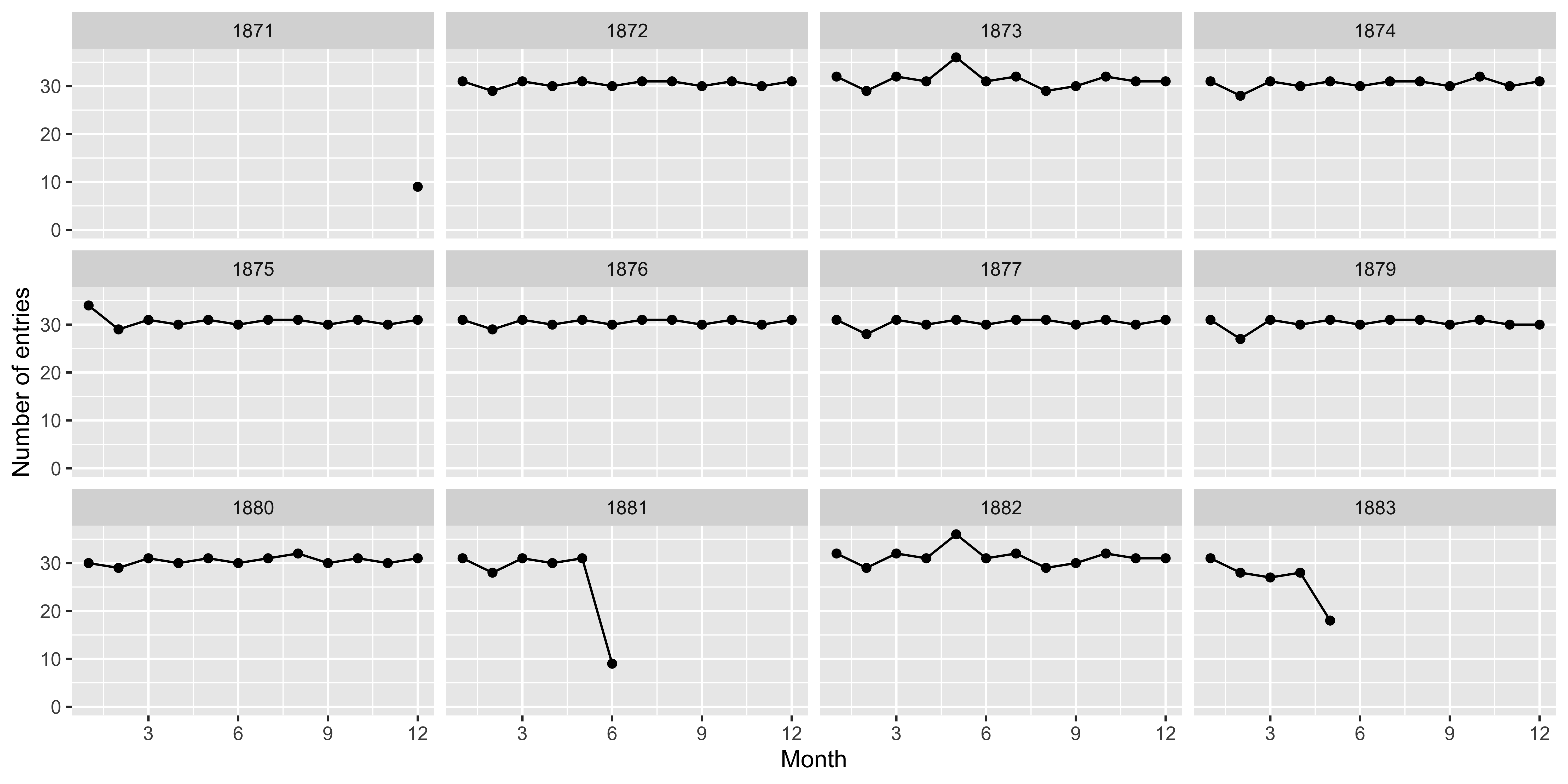
How often did Freeland write?
Where did Freeland go? Step by Step
Start with the dataset
journals_sub
#> # A tibble: 5,509 × 5
#>    date_mdy   journal_entry                                 location  year month
#>    <date>     <chr>                                         <chr>    <dbl> <dbl>
#>  1 1871-12-23 Was married at home in evening by William Ra… Winter …  1871    12
#>  2 1871-12-24 Went to meeting.                              NA        1871    12
#>  3 1871-12-25 Shooting match all day in the evening to Chr… Winter …  1871    12
#>  4 1871-12-26 About home at work jobbing.                   Winter …  1871    12
#>  5 1871-12-27 Work about home reed letter from N. H. Higgi… Winter …  1871    12
#>  6 1871-12-28 Work about home.                              Winter …  1871    12
#>  7 1871-12-29 To work in shop.                              Winter …  1871    12
#>  8 1871-12-30 To work in shop.                              Winter …  1871    12
#>  9 1871-12-31 Went to meeting.                              Winter …  1871    12
#> 10 1872-01-01 Work in shop.                                 Winter …  1872     1
#> # ℹ 5,499 more rows
Where did Freeland go? Step by Step
And then filter for only known locations
journals_sub %>%
    filter(is.na(location) == FALSE, location != "NA")
#> # A tibble: 3,164 × 5
#>    date_mdy   journal_entry                                 location  year month
#>    <date>     <chr>                                         <chr>    <dbl> <dbl>
#>  1 1871-12-23 Was married at home in evening by William Ra… Winter …  1871    12
#>  2 1871-12-25 Shooting match all day in the evening to Chr… Winter …  1871    12
#>  3 1871-12-26 About home at work jobbing.                   Winter …  1871    12
#>  4 1871-12-27 Work about home reed letter from N. H. Higgi… Winter …  1871    12
#>  5 1871-12-28 Work about home.                              Winter …  1871    12
#>  6 1871-12-29 To work in shop.                              Winter …  1871    12
#>  7 1871-12-30 To work in shop.                              Winter …  1871    12
#>  8 1871-12-31 Went to meeting.                              Winter …  1871    12
#>  9 1872-01-01 Work in shop.                                 Winter …  1872     1
#> 10 1872-01-02 Work in shop.                                 Winter …  1872     1
#> # ℹ 3,154 more rows- The function
filterlets you filter rows based on their values.
Where did Freeland go? Step by Step
And then separate_longer_delim so each location is on its own row
journals_sub %>%
    filter(is.na(location) == FALSE, location != "NA") %>%
    separate_longer_delim(location, delim = ", ")
#> # A tibble: 4,138 × 5
#>    date_mdy   journal_entry                                 location  year month
#>    <date>     <chr>                                         <chr>    <dbl> <dbl>
#>  1 1871-12-23 Was married at home in evening by William Ra… Winter …  1871    12
#>  2 1871-12-25 Shooting match all day in the evening to Chr… Winter …  1871    12
#>  3 1871-12-26 About home at work jobbing.                   Winter …  1871    12
#>  4 1871-12-27 Work about home reed letter from N. H. Higgi… Winter …  1871    12
#>  5 1871-12-28 Work about home.                              Winter …  1871    12
#>  6 1871-12-29 To work in shop.                              Winter …  1871    12
#>  7 1871-12-30 To work in shop.                              Winter …  1871    12
#>  8 1871-12-31 Went to meeting.                              Winter …  1871    12
#>  9 1872-01-01 Work in shop.                                 Winter …  1872     1
#> 10 1872-01-02 Work in shop.                                 Winter …  1872     1
#> # ℹ 4,128 more rows
Where did Freeland go? Step by Step
And then count the number of times he was at that location
journals_sub %>%
    filter(is.na(location) == FALSE, location != "NA") %>%
    separate_longer_delim(location, delim = ", ") %>%
    count(location)
#> # A tibble: 312 × 2
#>    location                     n
#>    <chr>                    <int>
#>  1 ""                           1
#>  2 " Northeast Harbor"          1
#>  3 "? Virgin"                   1
#>  4 "Albany Railroad Wharf"      9
#>  5 "Atlantic Wharf"             6
#>  6 "Azores/Western Islands"     1
#>  7 "Back Shore"                 1
#>  8 "Baker Island"              10
#>  9 "Bakers Island"              1
#> 10 "Bangor"                     5
#> # ℹ 302 more rows
Where did Freeland go? Step by Step
And then arrange the locations in descending order from most to least visited.
journals_sub %>%
    filter(is.na(location) == FALSE, location != "NA") %>%
    separate_longer_delim(location, delim = ", ") %>%
    count(location) %>%
    arrange(desc(n))
#> # A tibble: 312 × 2
#>    location            n
#>    <chr>           <int>
#>  1 Winter Harbor    2368
#>  2 West Gouldsboro   132
#>  3 Ellsworth          68
#>  4 Rockland           55
#>  5 Bar Harbor         44
#>  6 Leghorn            43
#>  7 Boston             42
#>  8 Prospect Harbor    39
#>  9 Cranberry Isles    37
#> 10 Calais             36
#> # ℹ 302 more rows
Where did Freeland go less? Step by Step
And then arrange the locations in ascending order from least to most visited.
journals_sub %>%
    filter(is.na(location) == FALSE, location != "NA") %>%
    separate_longer_delim(location, delim = ", ") %>%
    count(location) %>%
    arrange(n)
#> # A tibble: 312 × 2
#>    location                     n
#>    <chr>                    <int>
#>  1 ""                           1
#>  2 " Northeast Harbor"          1
#>  3 "? Virgin"                   1
#>  4 "Azores/Western Islands"     1
#>  5 "Back Shore"                 1
#>  6 "Bakers Island"              1
#>  7 "Bass Habor"                 1
#>  8 "Bishop and Clerks"          1
#>  9 "Block Island"               1
#> 10 "Bog Brook"                  1
#> # ℹ 302 more rows
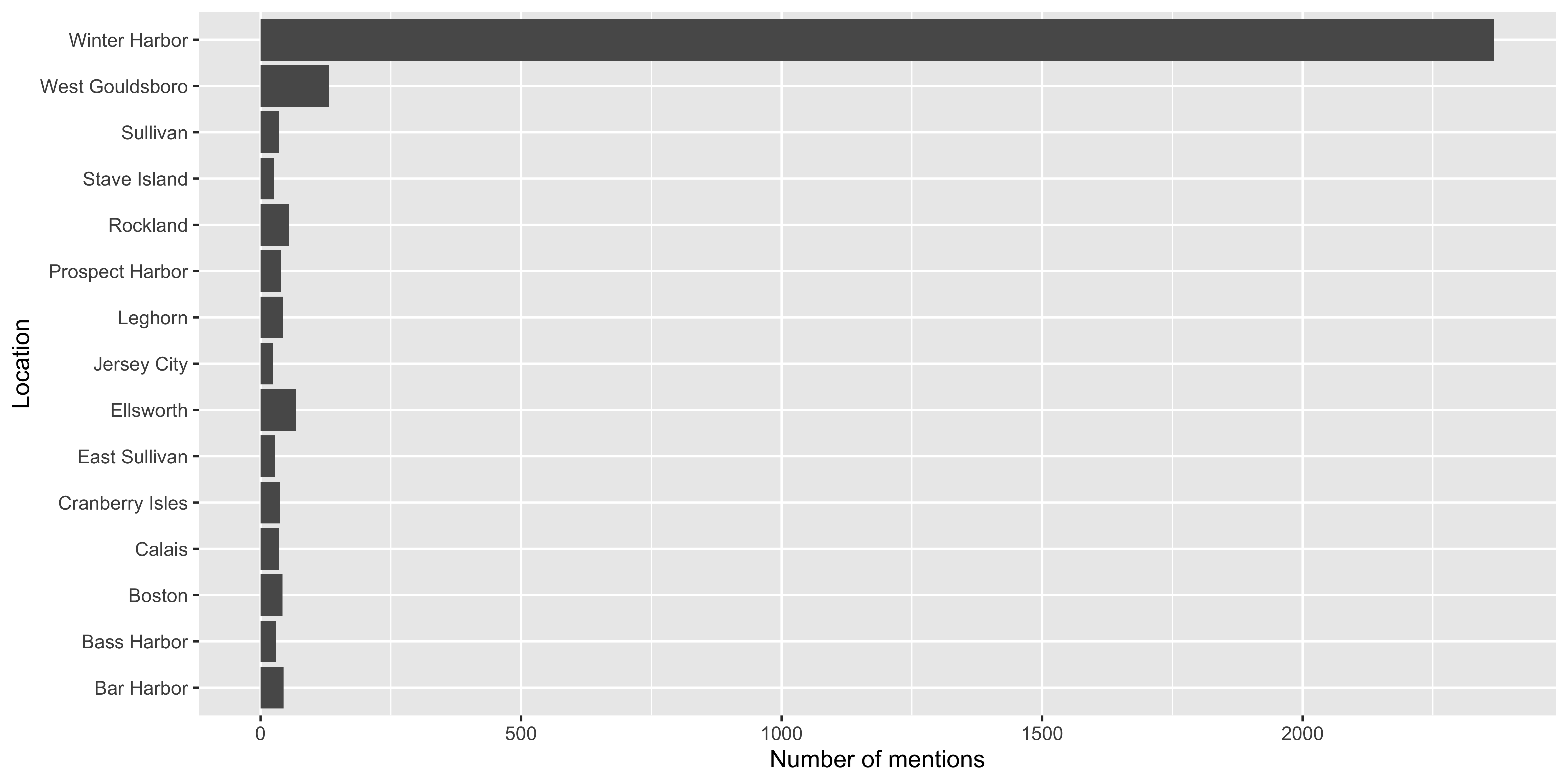
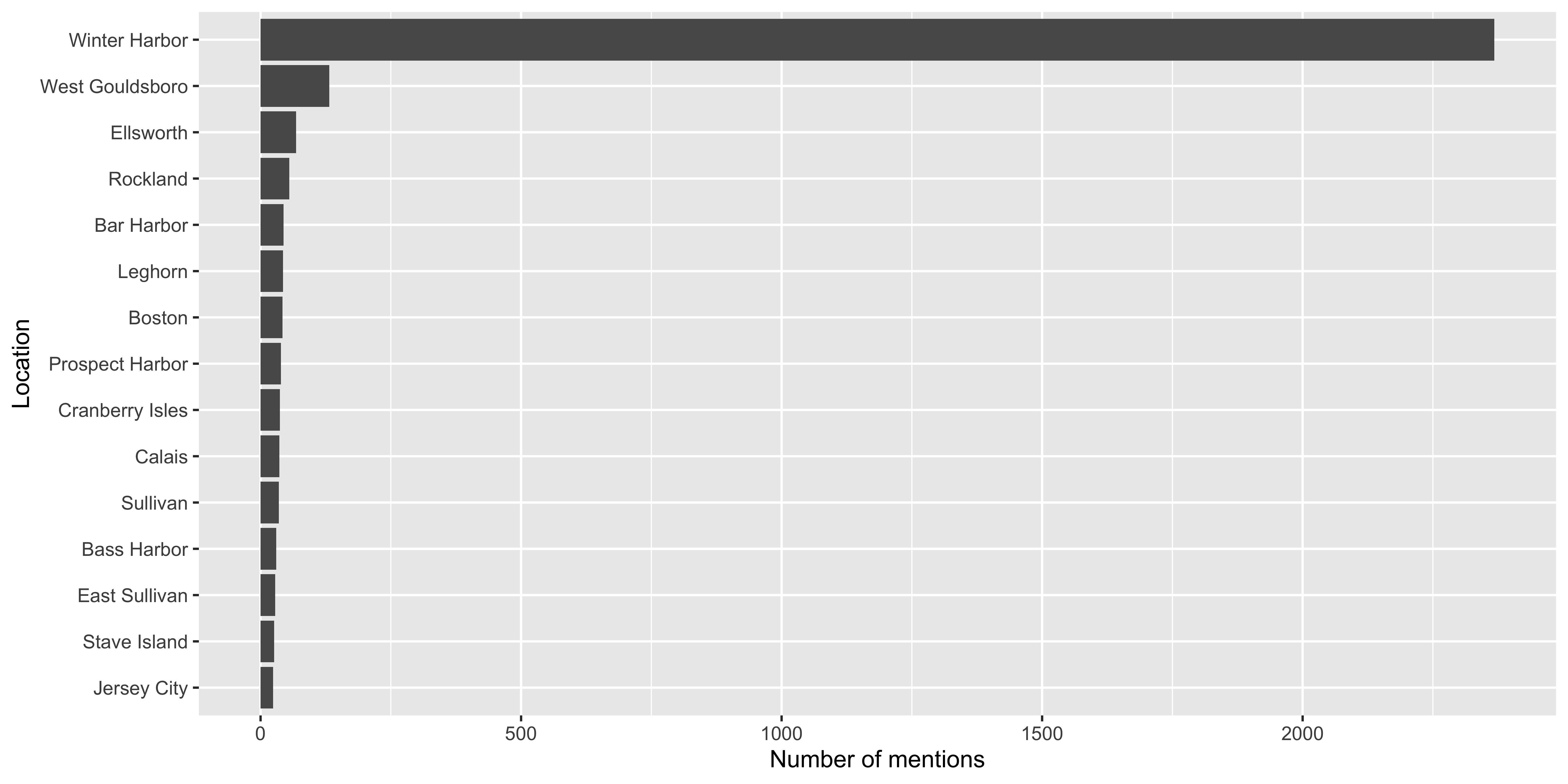
Plotting frequency of visits
(common_places <- journals_sub %>%
    filter(is.na(location) == FALSE, location != "NA") %>%
    separate_longer_delim(location, delim = ", ") %>%
    count(location) %>%
    slice_max(n, n = 15, with_ties = FALSE))
#> # A tibble: 15 × 2
#>    location            n
#>    <chr>           <int>
#>  1 Winter Harbor    2368
#>  2 West Gouldsboro   132
#>  3 Ellsworth          68
#>  4 Rockland           55
#>  5 Bar Harbor         44
#>  6 Leghorn            43
#>  7 Boston             42
#>  8 Prospect Harbor    39
#>  9 Cranberry Isles    37
#> 10 Calais             36
#> 11 Sullivan           35
#> 12 Bass Harbor        30
#> 13 East Sullivan      28
#> 14 Stave Island       26
#> 15 Jersey City        24
Plotting frequency of visits
- Learn about
ggplotin these slides and with these interactive tutorials
Plotting frequency of visits
Use distinct to detect mispellings and look at unique entries
journals_sub %>%
    separate_longer_delim(location, delim = ", ") %>%
    filter(str_detect(string = location, pattern = "Cranberry")) %>%
    distinct(location)
#> # A tibble: 4 × 1
#>   location
#>   <chr>
#> 1 "Cranberry Island"
#> 2 "Cranberry Isles"
#> 3 "Winter Harbor,Cranberry Isles"
#> 4 "Cranberry Isles "
Tidying words using case_when
journals_sub <- journals_sub %>%
    separate_rows(location, sep = ",") %>%
    mutate(location = case_when(location %in% c("Cranberry Isle", "Cranberry Island") ~ "Cranberry Isles",
                            TRUE ~ location))


journals_sub %>%
    filter(str_detect(string = location, pattern = "Cranberry")) %>%
    distinct(location)
#> # A tibble: 3 × 1
#>   location
#>   <chr>
#> 1 "Cranberry Isles"
#> 2 " Cranberry Isles"
#> 3 " Cranberry Isles "
Why are places still coming up as different?
We can use str_trim() to get rid of white space.
Your Turn: Fix Bass Harbor misspellings
Where did Freeland visit

How often did Freeland visit over time?
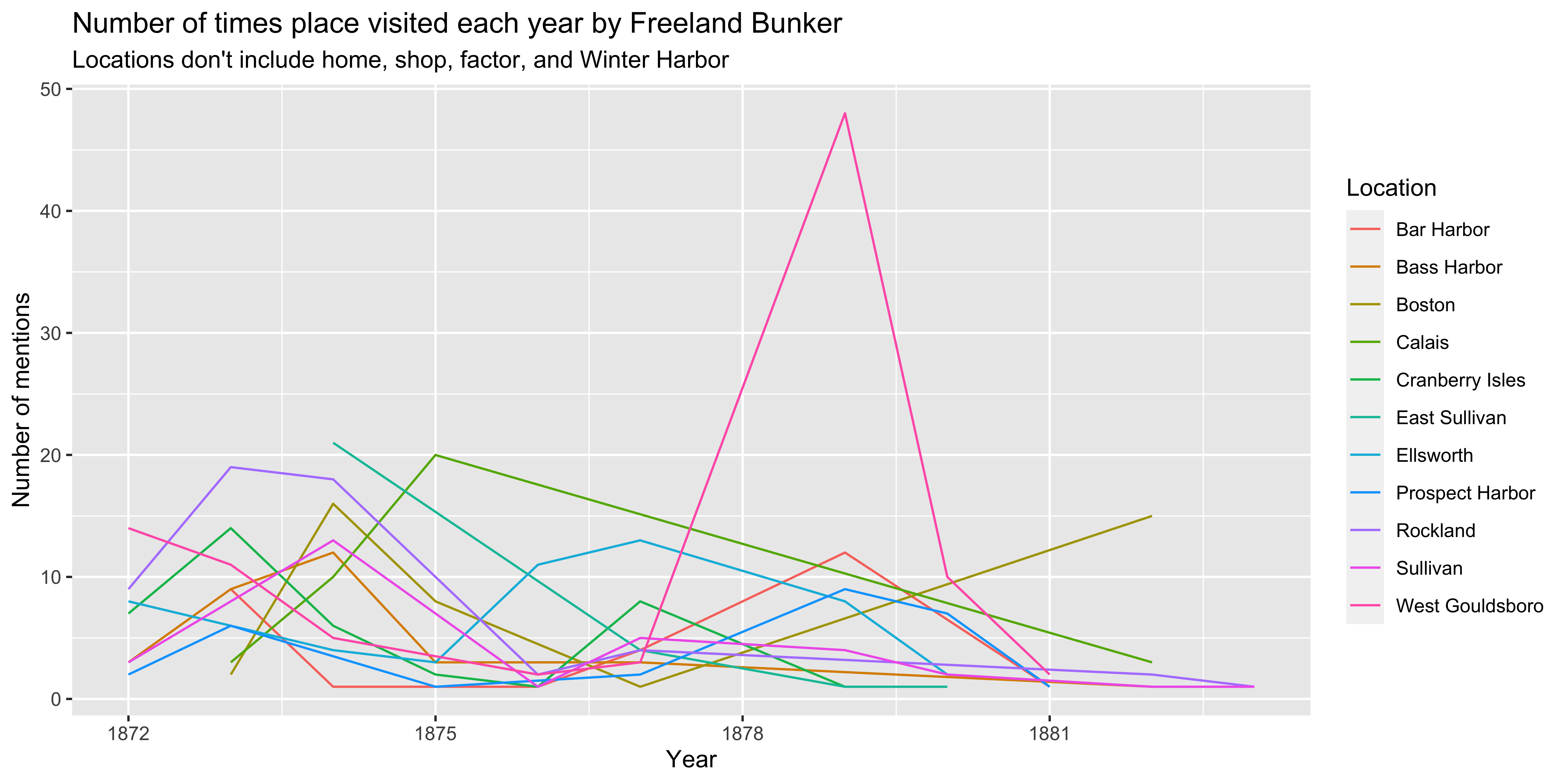
Use group_by to count yearly visits
(journals_loc_count <- journals_sub %>%
    filter(location %in% c("West Gouldsboro", "Ellsworth", "Rockland", "Bar Harbor", "Sullivan", "Calais", "Prospect Harbor", "East Sullivan", "Boston", "Bass Harbor", "Cranberry Isles")) %>%
    group_by(year) %>%
    count(location))
#> # A tibble: 76 × 3
#> # Groups:   year [12]
#>     year location            n
#>    <dbl> <chr>           <int>
#>  1  1872 Bass Harbor         3
#>  2  1872 Cranberry Isles     7
#>  3  1872 Ellsworth           8
#>  4  1872 Prospect Harbor     2
#>  5  1872 Rockland            9
#>  6  1872 Sullivan            3
#>  7  1872 West Gouldsboro    14
#>  8  1873 Bar Harbor          9
#>  9  1873 Bass Harbor         9
#> 10  1873 Boston              2
#> # ℹ 66 more rows
Plot Code

Your Turn
Where did Freeland visit during your journal year? Fill in the blanks to find out.
Creating maps using leaflet
We have location coordinates
We have a count of how often Freeland visited that location
(loc_count <- journals_sub %>%
    count(location) %>%
    arrange(desc(n)))
#> # A tibble: 308 × 2
#>    location            n
#>    <chr>           <int>
#>  1 Winter Harbor    2369
#>  2 West Gouldsboro   132
#>  3 Ellsworth          68
#>  4 Rockland           55
#>  5 Bar Harbor         44
#>  6 Leghorn            43
#>  7 Boston             42
#>  8 Cranberry Isles    39
#>  9 Prospect Harbor    39
#> 10 Calais             36
#> # ℹ 298 more rows
We can combine two data sets using a join
(loc_df <- loc_count %>%
left_join(location_coordinates, by = "location") %>%
drop_na(latitude) %>%
mutate(latitude = as.numeric(latitude),
longitude = as.numeric(longitude))
)
#> # A tibble: 99 × 16
#> location n Instructions official_name_check.…¹ latitude longitude
#> <chr> <int> <chr> <chr> <dbl> <dbl>
#> 1 Winter Harbor 2369 <NA> yes 44.4 -68.1
#> 2 West Gouldsboro 132 <NA> yes 44.5 -68.1
#> 3 Ellsworth 68 <NA> yes 44.5 -68.4
#> 4 Rockland 55 <NA> yes 44.1 -69.1
#> 5 Bar Harbor 44 <NA> yes 44.4 -68.2
#> 6 Leghorn 43 <NA> yes 43.6 10.3
#> 7 Boston 42 location_dro… yes 42.4 -71.1
#> 8 Cranberry Isles 39 <NA> yes 44.3 -68.3
#> 9 Prospect Harbor 39 <NA> yes 44.4 -68.0
#> 10 Calais 36 <NA> yes 45.2 -67.3
#> # ℹ 89 more rows
#> # ℹ abbreviated name: ¹official_name_check...3
#> # ℹ 10 more variables: date_mentioned_location <chr>, location_notes <chr>,
#> # initials...8 <chr>, local_place_list <chr>, official_name_check...10 <chr>,
#> # local_place_latitude <dbl>, local_place_longitude <dbl>,
#> # date_mentioned_local <chr>, local_place_notes <chr>, initials...15 <chr>Where did Freeland go?
Where did Freeland go?
Homework
- Double check a location’s coordinates or
- Look up two locations and add 2 more sets of coordinates to the location excel file. Add your initials to the excel spreadsheet.
- Re-upload the location data
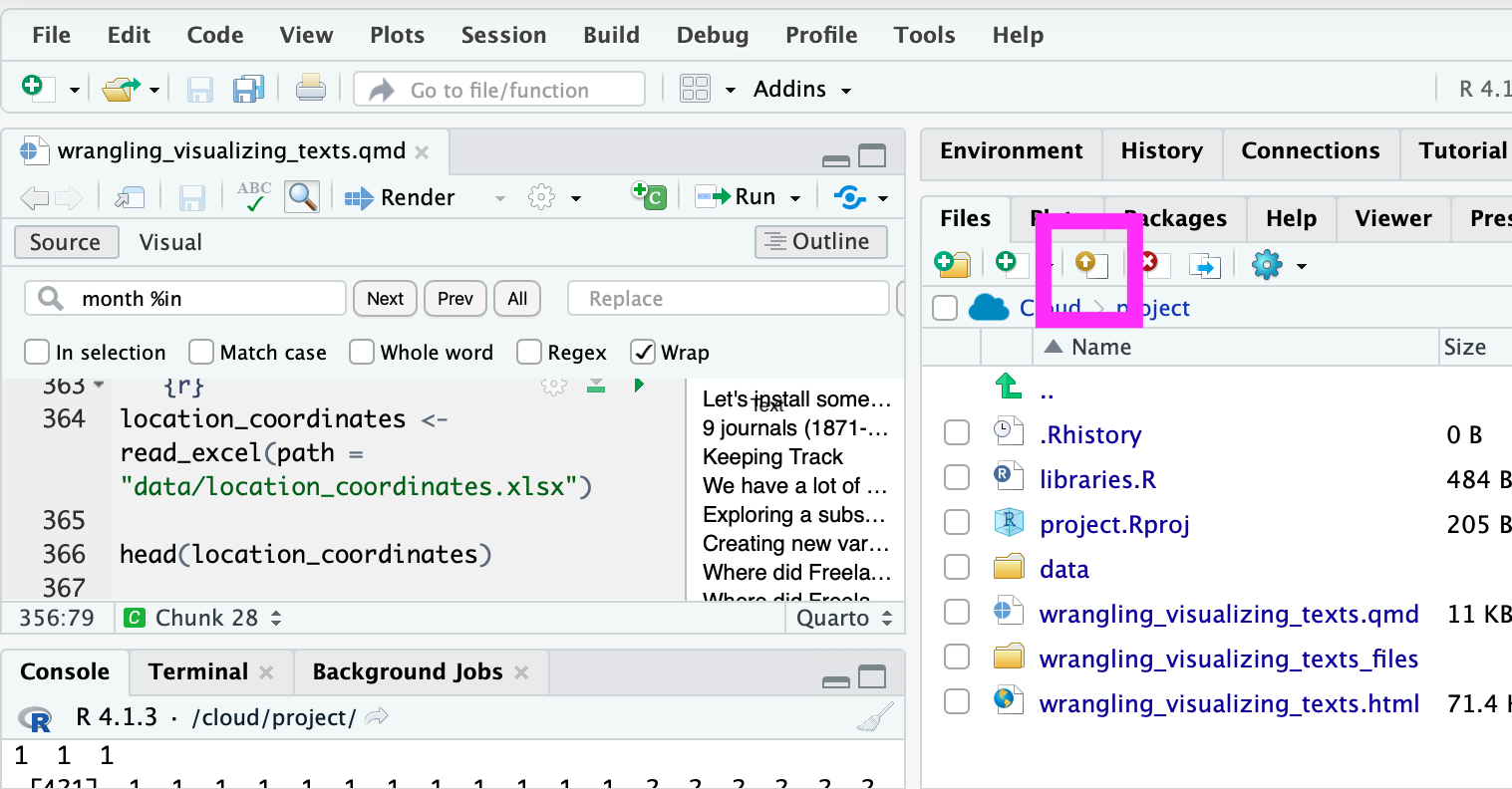
- Rerun the leaflet map to see the map expand
Thanks!
Slides created with Quarto