Comparing Historical Texts

USING TIDY DATA PRINCIPLES

by Laurie Baker

Acknowledgements

Slide Structure, Content, and Design adapted from Julia Silge

Let’s install some packages

install.packages(c("tidyverse", 
                   "tidytext",
                   "stopwords",
                   "widyr",
                   "tidygraph",
                   "tidylo",
                   "ggraph",
                   "wordcloud"))

WHAT IS A DOCUMENT ABOUT? 🤔

What is a document about?

Term frequency
Inverse document frequency

\[idf(\text{term}) = \ln{\left(\frac{n_{\text{documents}}}{n_{\text{documents containing term}}}\right)}\]

tf-idf is about comparing documents within a collection.

Understanding tf-idf

Make a collection (corpus) for yourself!


journal_1871_1872$journal <- 1
journal_1873$journal <- 2
journal_1874$journal <- 3
journal_1875$journal <- 4
journal_1876$journal <- 5
journal_1877$journal <- 6
journal_1878$journal <- 7
journal_1879$journal <- 8
journal_1880$journal <- 9

journals <- dplyr::bind_rows(journal_1871_1872, journal_1873, journal_1874, 
                             journal_1875, journal_1876, journal_1877, 
                             journal_1878, journal_1879, journal_1880)

Understanding tf-idf

Make a collection (corpus) for yourself!

journals %>%
    select(date_mdy, journal_entry, location)
#> # A tibble: 3,951 × 3
#>    date_mdy   journal_entry                                             location
#>    <chr>      <chr>                                                     <chr>   
#>  1 12/23/1871 Was married at home in evening by William Rand Esqr.      home    
#>  2 12/24/1871 Went to meeting.                                          NA      
#>  3 12/25/1871 Shooting match all day in the evening to Christmas tree … hall    
#>  4 12/26/1871 About home at work fobbing.                               home    
#>  5 12/27/1871 Work about home reed letter from N. H. Higgins Ins agt.   home    
#>  6 12/28/1871 Work about home.                                          home    
#>  7 12/29/1871 To work in shop.                                          shop    
#>  8 12/30/1871 To work in shop.                                          shop    
#>  9 12/31/1871 Went to meeting.                                          NA      
#> 10 1/1/1872   Work in shop.                                             shop    
#> # ℹ 3,941 more rows

Counting word frequencies

library(tidyverse)
library(tidytext)

(journal_words <- journals %>%
    unnest_tokens(word, journal_entry) %>%
    count(journal, word, sort = TRUE))
#> # A tibble: 9,200 × 3
#>    journal word      n
#>      <dbl> <chr> <int>
#>  1       8 the     868
#>  2       7 the     701
#>  3       4 the     672
#>  4       6 the     644
#>  5       7 <NA>    640
#>  6       9 the     562
#>  7       2 the     539
#>  8       3 the     537
#>  9       5 the     523
#> 10       4 wind    421
#> # ℹ 9,190 more rows

What do the columns of journal_words tell us?

Calculating tf-idf

journal_tf_idf <- journal_words %>%
    bind_tf_idf(word, journal, n)

Calculating tf-idf

journal_tf_idf
#> # A tibble: 9,200 × 6
#>    journal word      n     tf   idf tf_idf
#>      <dbl> <chr> <int>  <dbl> <dbl>  <dbl>
#>  1       8 the     868 0.0895     0      0
#>  2       7 the     701 0.0741     0      0
#>  3       4 the     672 0.0881     0      0
#>  4       6 the     644 0.0907     0      0
#>  5       7 <NA>    640 0.0677    NA     NA
#>  6       9 the     562 0.0634     0      0
#>  7       2 the     539 0.0825     0      0
#>  8       3 the     537 0.0866     0      0
#>  9       5 the     523 0.0861     0      0
#> 10       4 wind    421 0.0552     0      0
#> # ℹ 9,190 more rows

That’s… super exciting???

Calculating tf-idf

What do you predict will happen if we run the following code? 🤔

journal_tf_idf %>%
    arrange(-tf_idf)

Calculating tf-idf

What do you predict will happen if we run the following code? 🤔

journal_tf_idf %>%
    arrange(-tf_idf)
#> # A tibble: 9,200 × 6
#>    journal word            n      tf   idf tf_idf
#>      <dbl> <chr>       <int>   <dbl> <dbl>  <dbl>
#>  1       9 thermometer   357 0.0403  0.811 0.0327
#>  2       7 thermometer   351 0.0371  0.811 0.0301
#>  3       9 degrees       239 0.0270  1.10  0.0296
#>  4       8 thermometer   353 0.0364  0.811 0.0295
#>  5       8 degrees       200 0.0206  1.10  0.0227
#>  6       7 degrees       166 0.0176  1.10  0.0193
#>  7       1 lobsters       26 0.00727 2.20  0.0160
#>  8       1 lbs            36 0.0101  1.50  0.0151
#>  9       1 factory        32 0.00895 1.50  0.0135
#> 10       9 troll          46 0.00519 2.20  0.0114
#> # ℹ 9,190 more rows

Calculating tf-idf

U N S C R A M B L E

group_by(journal) %>%

journal_tf_idf %>%

slice_max(tf_idf, n = 10) %>%

ggplot(aes(tf_idf, fct_reorder(word, tf_idf), fill = journal)) +

facet_wrap(vars(journal), scales = “free”)

geom_col(show.legend = FALSE) +

Calculating tf-idf

journal_tf_idf %>%
    group_by(journal) %>%
    slice_max(tf_idf, n = 10) %>%
    ggplot(aes(tf_idf, fct_reorder(word, tf_idf), fill = journal)) +
    geom_col(show.legend = FALSE) +
    facet_wrap(vars(journal), scales = "free") +
    scale_x_continuous(expand = c(0,0)) +
    labs(y = NULL, x = "tf-idf", title = "Highest tf-idf words in Freeland Bunker's Journals")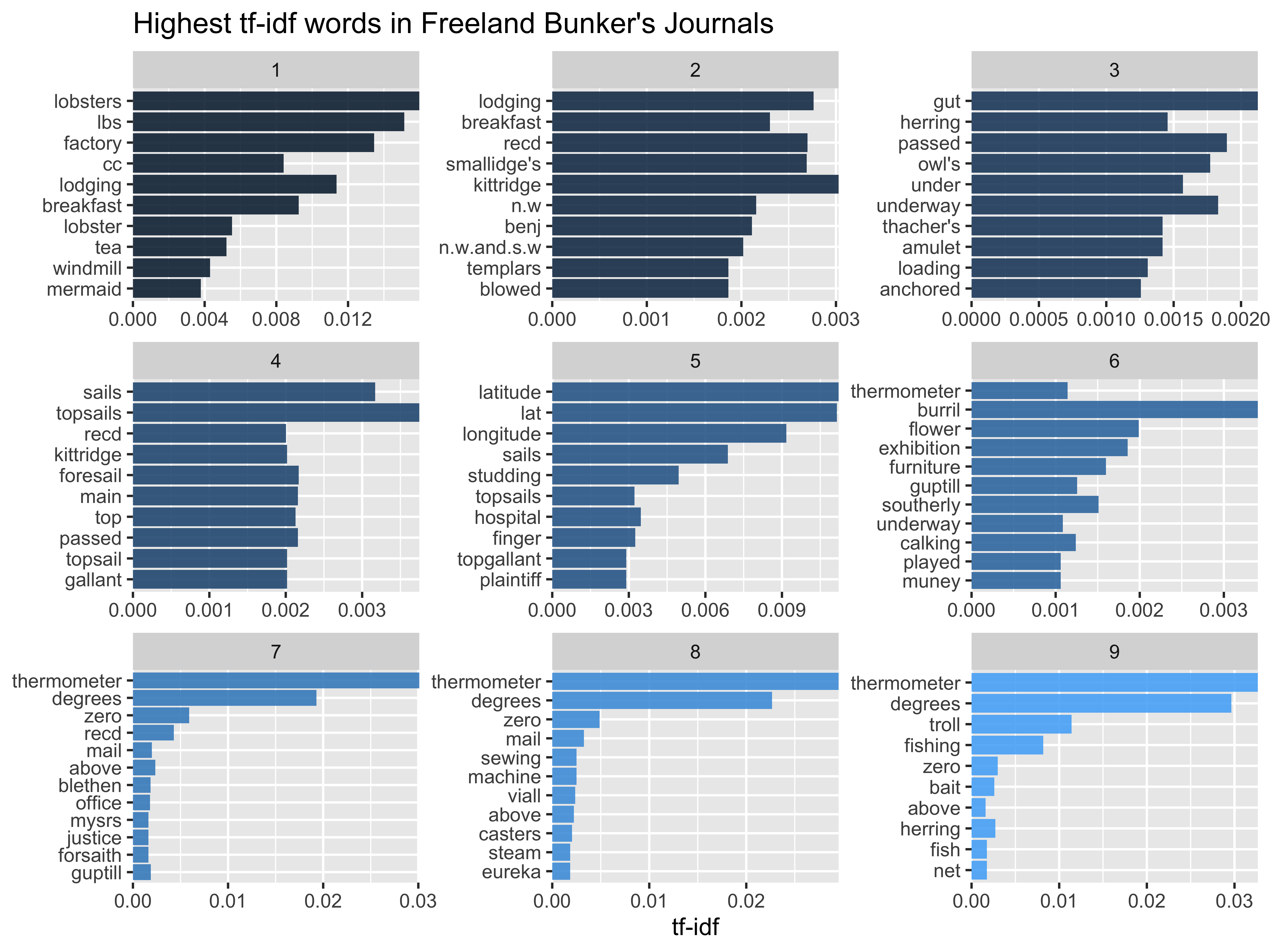

More insight from bigrams!

(tidy_ngram <- journals %>%
    unnest_tokens(bigram, journal_entry, token = "ngrams", n = 2) %>% 
    drop_na(bigram) %>%
    select(journal, bigram, date_mdy, location))
#> # A tibble: 61,167 × 4
#>    journal bigram       date_mdy   location
#>      <dbl> <chr>        <chr>      <chr>   
#>  1       1 was married  12/23/1871 home    
#>  2       1 married at   12/23/1871 home    
#>  3       1 at home      12/23/1871 home    
#>  4       1 home in      12/23/1871 home    
#>  5       1 in evening   12/23/1871 home    
#>  6       1 evening by   12/23/1871 home    
#>  7       1 by william   12/23/1871 home    
#>  8       1 william rand 12/23/1871 home    
#>  9       1 rand esqr    12/23/1871 home    
#> 10       1 went to      12/24/1871 NA      
#> # ℹ 61,157 more rows

N-grams… and beyond! 🚀

tidy_ngram %>%
    count(bigram, sort = TRUE)
#> # A tibble: 19,411 × 2
#>    bigram             n
#>    <chr>          <int>
#>  1 the wind        2760
#>  2 in the           735
#>  3 wind north       572
#>  4 went to          557
#>  5 wind southerly   543
#>  6 all day          483
#>  7 north west       402
#>  8 wind south       381
#>  9 the afternoon    292
#> 10 south west       275
#> # ℹ 19,401 more rows

Freeland wants to know…

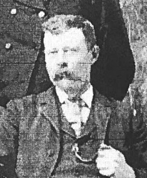
Can we use an anti_join() now to remove stop words?

Yes! ✅
No ☹️

N-grams… and beyond! 🚀

bigram_counts <- tidy_ngram %>%
    separate(bigram, c("word1", "word2"), sep = " ") %>%
    filter(!word1 %in% stop_words$word,
           !word2 %in% stop_words$word) %>%
    count(word1, word2, sort = TRUE)

So many wind directions…! 🚀

bigram_counts
#> # A tibble: 7,243 × 3
#>    word1 word2           n
#>    <chr> <chr>       <int>
#>  1 wind  north         572
#>  2 wind  southerly     543
#>  3 north west          402
#>  4 wind  south         381
#>  5 south west          275
#>  6 wrote letter        263
#>  7 wind  easterly      243
#>  8 west  thermometer   186
#>  9 wind  westerly      182
#> 10 fresh breeze        175
#> # ℹ 7,233 more rows

How did Freeland refer to wind?

library(wordcloud)
bigram_counts %>%
    filter(str_detect(string = word1, pattern = "wind|Wind")) %>% 
    with(wordcloud::wordcloud(word2, n, random.order = FALSE, max.words = 50, colors = brewer.pal(8,"Dark2")))

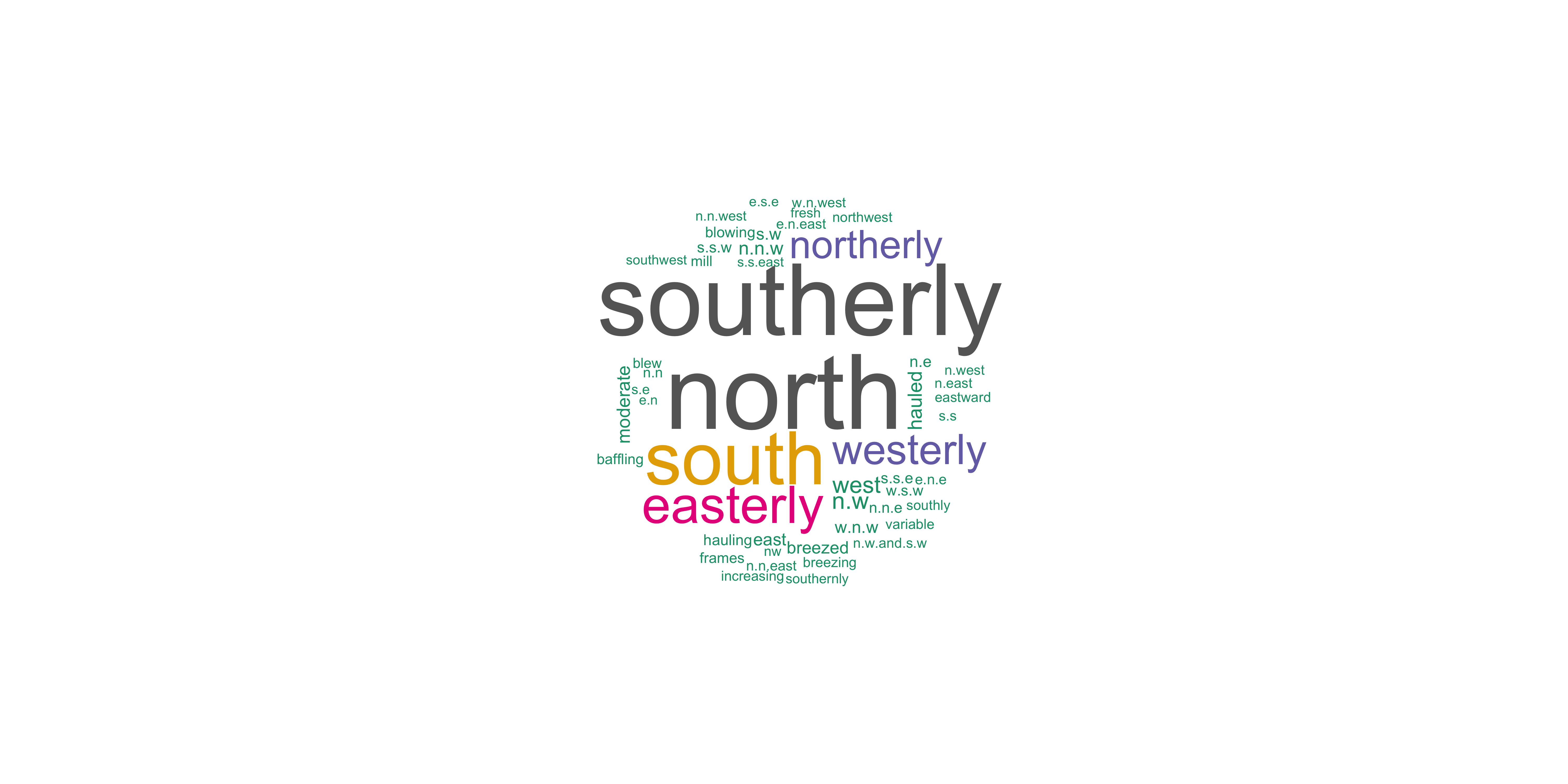
Let’s remove stopwords, wind, and more

words_to_remove <- c("wind", "thermometer", "north", "west", "south", "east", "degrees", "afternoon", "morning")

bigram_counts <- tidy_ngram %>%
    separate(bigram, c("word1", "word2"), sep = " ") %>%
    filter(!word1 %in% c(stop_words$word, words_to_remove),
           !word2 %in% c(stop_words$word, words_to_remove)) %>%
    count(word1, word2, sort = TRUE)

What can you do with n-grams?

tf-idf of n-grams
weighted log odds of n-grams
network analysis
negation

Network analysis

library(widyr)
library(ggraph)
library(tidygraph)

bigram_graph <- bigram_counts %>%
    filter(n > 15) %>%
    as_tbl_graph()

Network analysis

bigram_graph
#> # A tbl_graph: 106 nodes and 104 edges
#> #
#> # A directed multigraph with 20 components
#> #
#> # A tibble: 106 × 1
#>   name     
#>   <chr>    
#> 1 north    
#> 2 south    
#> 3 wrote    
#> 4 west     
#> 5 fresh    
#> 6 southerly
#> # ℹ 100 more rows
#> #
#> # A tibble: 104 × 3
#>    from    to     n
#>   <int> <int> <int>
#> 1     1     4   402
#> 2     2     4   275
#> 3     3    14   263
#> # ℹ 101 more rows

Freeland wants to know…

Is bigram_graph a tidy dataset?

Yes ☑️
No 🚫

Network analysis

bigram_graph %>%
    ggraph(layout = "kk") +
    geom_edge_link(aes(edge_alpha = n), 
                   show.legend = FALSE, 
                   arrow = arrow(length = unit(1.5, 'mm')), 
                   start_cap = circle(3, 'mm'),
                   end_cap = circle(3, 'mm')) +
    geom_node_text(aes(label = name)) + 
    theme_graph()

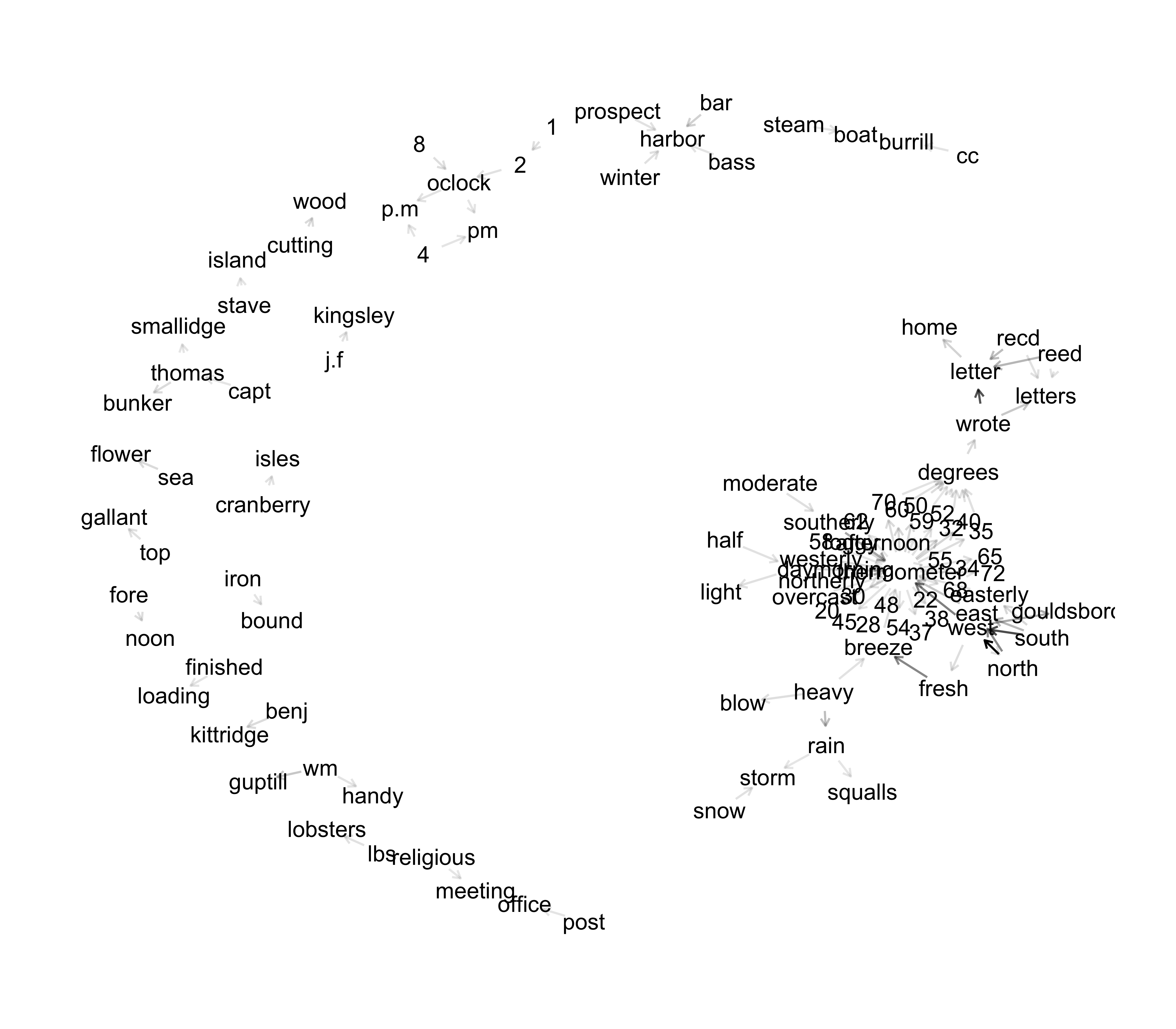
What can we learn from trigrams?

(tidy_trigram <- journals %>%
    unnest_tokens(trigram, journal_entry, token = "ngrams", n = 3) %>% 
    drop_na(trigram) %>%
    select(journal, trigram, date_mdy, location))
#> # A tibble: 57,904 × 4
#>    journal trigram            date_mdy   location
#>      <dbl> <chr>              <chr>      <chr>   
#>  1       1 was married at     12/23/1871 home    
#>  2       1 married at home    12/23/1871 home    
#>  3       1 at home in         12/23/1871 home    
#>  4       1 home in evening    12/23/1871 home    
#>  5       1 in evening by      12/23/1871 home    
#>  6       1 evening by william 12/23/1871 home    
#>  7       1 by william rand    12/23/1871 home    
#>  8       1 william rand esqr  12/23/1871 home    
#>  9       1 went to meeting    12/24/1871 NA      
#> 10       1 shooting match all 12/25/1871 hall    
#> # ℹ 57,894 more rows

Trigram counts

words_to_remove <- c("wind", "thermometer", "north", "west", "south", "east", "degrees", "afternoon", "morning")

(trigram_counts <- tidy_trigram %>%
    separate(trigram, c("word1", "word2", "word3"), sep = " ") %>%
    filter(!word1 %in% c(stop_words$word, words_to_remove),
           !word2 %in% c(stop_words$word, words_to_remove),
           !word3 %in% c(stop_words$word, words_to_remove)) %>%
    count(word1, word2, word3, sort = TRUE))
#> # A tibble: 3,881 × 4
#>    word1    word2   word3          n
#>    <chr>    <chr>   <chr>      <int>
#>  1 wrote    letter  home          44
#>  2 steam    boat    wharf         14
#>  3 top      gallant sail          12
#>  4 top      gallant sails         12
#>  5 1        2       day           11
#>  6 easterly fresh   breeze        11
#>  7 post     office  department    11
#>  8 capt     thomas  bunker        10
#>  9 home     cutting wood           9
#> 10 main     top     gallant        9
#> # ℹ 3,871 more rows

Thanks!

@LaurieLBaker

lauriebaker@rbind.io

Additional Slides

WHAT IS A DOCUMENT ABOUT - other methods? 🤔

What is a document about?

Term frequency
Inverse document frequency

Weighted log odds ⚖️

Log odds ratio expresses probabilities
Weighting helps deal with power law distribution

Weighted log odds ⚖️

library(tidylo)
journal_words %>%
    bind_log_odds(journal, word, n) %>%
    arrange(-log_odds_weighted)
#> # A tibble: 9,200 × 4
#>    journal word            n log_odds_weighted
#>      <dbl> <chr>       <int>             <dbl>
#>  1       7 <NA>          640              47.8
#>  2       9 thermometer   357              27.5
#>  3       9 degrees       239              27.1
#>  4       8 thermometer   353              26.8
#>  5       7 thermometer   351              26.8
#>  6       8 degrees       200              25.1
#>  7       6 <NA>            2              23.9
#>  8       7 degrees       166              23.6
#>  9       6 thermometer    10              17.5
#> 10       9 troll          46              14.4
#> # ℹ 9,190 more rows

Weighted log odds can distinguish between words that are used in all texts.