Text Mining

USING TIDY DATA PRINCIPLES

by Julia Silge adapted with a COA twist by Laurie Baker

Acknowledgements

@juliasilge

@juliasilge

youtube.com/juliasilge

juliasilge.com

tidytextmining.com

Let’s install some packages

install.packages(c("tidyverse", 
                   "tidytext",
                   "stopwords",
                   "gutenbergr"))

What do we mean by tidy text?

text <- c("Tell all the truth but tell it slant —",
          "Success in Circuit lies",
          "Too bright for our infirm Delight",
          "The Truth's superb surprise",
          "As Lightning to the Children eased",
          "With explanation kind",
          "The Truth must dazzle gradually",
          "Or every man be blind —")

text
#> [1] "Tell all the truth but tell it slant —"
#> [2] "Success in Circuit lies"               
#> [3] "Too bright for our infirm Delight"     
#> [4] "The Truth's superb surprise"           
#> [5] "As Lightning to the Children eased"    
#> [6] "With explanation kind"                 
#> [7] "The Truth must dazzle gradually"       
#> [8] "Or every man be blind —"

What do we mean by tidy text?

library(tidyverse)

text_df <- tibble(line = 1:8, text = text)

text_df
#> # A tibble: 8 × 2
#>    line text                                  
#>   <int> <chr>                                 
#> 1     1 Tell all the truth but tell it slant —
#> 2     2 Success in Circuit lies               
#> 3     3 Too bright for our infirm Delight     
#> 4     4 The Truth's superb surprise           
#> 5     5 As Lightning to the Children eased    
#> 6     6 With explanation kind                 
#> 7     7 The Truth must dazzle gradually       
#> 8     8 Or every man be blind —

What do we mean by tidy text?

library(tidytext)

text_df %>%
    unnest_tokens(word, text)
#> # A tibble: 41 × 2
#>     line word   
#>    <int> <chr>  
#>  1     1 tell   
#>  2     1 all    
#>  3     1 the    
#>  4     1 truth  
#>  5     1 but    
#>  6     1 tell   
#>  7     1 it     
#>  8     1 slant  
#>  9     2 success
#> 10     2 in     
#> # ℹ 31 more rows

Jane wants to know…

A tidy text dataset typically has

• more
• fewer

rows than the original, non-tidy text dataset.

Gathering more data

You can access the full text of many public domain works from Project Gutenberg using the gutenbergr package.

library(gutenbergr)
gutenberg_works() %>%
  filter(title == "Anne of Green Gables")
#> # A tibble: 1 × 8
#>   gutenberg_id title     author gutenberg_author_id language gutenberg_bookshelf
#>          <int> <chr>     <chr>                <int> <chr>    <chr>              
#> 1           45 Anne of … Montg…                  36 en       Children's Literat…
#> # ℹ 2 more variables: rights <chr>, has_text <lgl>

my_mirror <- gutenberg_get_mirror()
full_text <- gutenberg_download(45, mirror = my_mirror)

https://docs.ropensci.org/gutenbergr/

Time to tidy your text!

tidy_book <- full_text %>%
    mutate(line = row_number()) %>%
    unnest_tokens(word, text)         

glimpse(tidy_book)
#> Rows: 0
#> Columns: 3
#> $ gutenberg_id <int> 
#> $ line         <int> 
#> $ word         <chr>

What are the most common words?

What do you predict will happen if we run the following code? 🤔

tidy_book %>%
    count(word, sort = TRUE)

What are the most common words?

What do you predict will happen if we run the following code? 🤔

tidy_book %>%
    count(word, sort = TRUE)
#> # A tibble: 0 × 2
#> # ℹ 2 variables: word <chr>, n <int>

Stop words

get_stopwords()
#> # A tibble: 175 × 2
#>    word      lexicon 
#>    <chr>     <chr>   
#>  1 i         snowball
#>  2 me        snowball
#>  3 my        snowball
#>  4 myself    snowball
#>  5 we        snowball
#>  6 our       snowball
#>  7 ours      snowball
#>  8 ourselves snowball
#>  9 you       snowball
#> 10 your      snowball
#> # ℹ 165 more rows

Stop words

get_stopwords(language = "es")
#> # A tibble: 308 × 2
#>    word  lexicon 
#>    <chr> <chr>   
#>  1 de    snowball
#>  2 la    snowball
#>  3 que   snowball
#>  4 el    snowball
#>  5 en    snowball
#>  6 y     snowball
#>  7 a     snowball
#>  8 los   snowball
#>  9 del   snowball
#> 10 se    snowball
#> # ℹ 298 more rows

Stop words

get_stopwords(language = "fr")
#> # A tibble: 164 × 2
#>    word  lexicon 
#>    <chr> <chr>   
#>  1 au    snowball
#>  2 aux   snowball
#>  3 avec  snowball
#>  4 ce    snowball
#>  5 ces   snowball
#>  6 dans  snowball
#>  7 de    snowball
#>  8 des   snowball
#>  9 du    snowball
#> 10 elle  snowball
#> # ℹ 154 more rows

Stop words

get_stopwords(source = "smart")
#> # A tibble: 571 × 2
#>    word        lexicon
#>    <chr>       <chr>  
#>  1 a           smart  
#>  2 a's         smart  
#>  3 able        smart  
#>  4 about       smart  
#>  5 above       smart  
#>  6 according   smart  
#>  7 accordingly smart  
#>  8 across      smart  
#>  9 actually    smart  
#> 10 after       smart  
#> # ℹ 561 more rows

What are the most common words?

U N S C R A M B L E

anti_join(get_stopwords(source = “smart”)) %>%

tidy_book %>%

count(word, sort = TRUE) %>%

geom_col() +

slice_max(n, n = 20) %>%

ggplot(aes(n, fct_reorder(word, n))) +

What are the most common words?

tidy_book %>%
    anti_join(get_stopwords(source = "smart")) %>%
    count(word, sort = TRUE) %>%
    slice_max(n, n = 20) %>%
    ggplot(aes(n, fct_reorder(word, n))) +  
    geom_col()

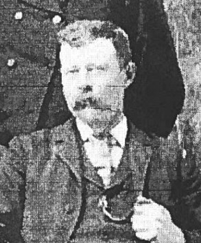
The Freeland Bunker Diaries

Currently 9 journals transcribed from 1871-1880

library(readxl)
journal_1871_1872 <- read_excel("data/journal_1871_1872.xlsx")
journal_1871_1872 %>%
    select(date_mdy, month, journal_entry) %>%
    head()
#> # A tibble: 6 × 3
#>   date_mdy   month    journal_entry                                             
#>   <chr>      <chr>    <chr>                                                     
#> 1 12/23/1871 December Was married at home in evening by William Rand Esqr.      
#> 2 12/24/1871 December Went to meeting.                                          
#> 3 12/25/1871 December Shooting match all day in the evening to Christmas tree a…
#> 4 12/26/1871 December About home at work jobbing.                               
#> 5 12/27/1871 December Work about home reed letter from N. H. Higgins Ins agt.   
#> 6 12/28/1871 December Work about home.

All Journals

journal_1873 <- read_excel("data/journal_1873.xlsx")
journal_1874 <- read_excel("data/journal_1874.xlsx")
journal_1875 <- read_excel("data/journal_1875.xlsx")
journal_1876 <- read_excel("data/journal_1876.xlsx")
journal_1877 <- read_excel("data/journal_1877.xlsx")
journal_1878 <- read_excel("data/journal_1878.xlsx")
journal_1879 <- read_excel("data/journal_1879.xlsx")
journal_1880 <- read_excel("data/journal_1880.xlsx")

Keeping Track

# We want to keep track of the journals

journal_1871_1872$journal <- 1
journal_1873$journal <- 2
journal_1874$journal <- 3
journal_1875$journal <- 4
journal_1876$journal <- 5
journal_1877$journal <- 6
journal_1878$journal <- 7
journal_1879$journal <- 8
journal_1880$journal <- 9

journals <- dplyr::bind_rows(journal_1871_1872, journal_1873, journal_1874, 
                             journal_1875, journal_1876, journal_1877, 
                             journal_1878, journal_1879, journal_1880)

Tidy Journals

library(lubridate)
(tidy_journal <- journals %>%
    select(date_mdy, month, journal_entry, journal) %>%
    mutate(date_mdy = mdy(date_mdy)) %>%
    mutate(year = year(date_mdy)) %>%
    unnest_tokens(word, journal_entry)  %>%
    mutate(word = case_when(word %in% c("reed", "read") ~ "received",
                            TRUE ~ word)))
#> # A tibble: 65,125 × 5
#>    date_mdy   month    journal  year word   
#>    <date>     <chr>      <dbl> <dbl> <chr>  
#>  1 1871-12-23 December       1  1871 was    
#>  2 1871-12-23 December       1  1871 married
#>  3 1871-12-23 December       1  1871 at     
#>  4 1871-12-23 December       1  1871 home   
#>  5 1871-12-23 December       1  1871 in     
#>  6 1871-12-23 December       1  1871 evening
#>  7 1871-12-23 December       1  1871 by     
#>  8 1871-12-23 December       1  1871 william
#>  9 1871-12-23 December       1  1871 rand   
#> 10 1871-12-23 December       1  1871 esqr   
#> # ℹ 65,115 more rows

Most common words

tidy_journal %>%
    count(word, sort = TRUE)
#> # A tibble: 4,083 × 2
#>    word            n
#>    <chr>       <int>
#>  1 the          5119
#>  2 wind         3052
#>  3 and          2302
#>  4 in           2181
#>  5 to           1959
#>  6 at           1421
#>  7 thermometer  1071
#>  8 of            949
#>  9 west          932
#> 10 went          910
#> # ℹ 4,073 more rows

Removing stop words

tidy_journal %>%
    anti_join(get_stopwords(source = "smart")) %>%
    count(word, sort = TRUE) %>%
    slice_max(n, n = 20) %>%
    ggplot(aes(n, fct_reorder(word, n))) +  
    geom_col()

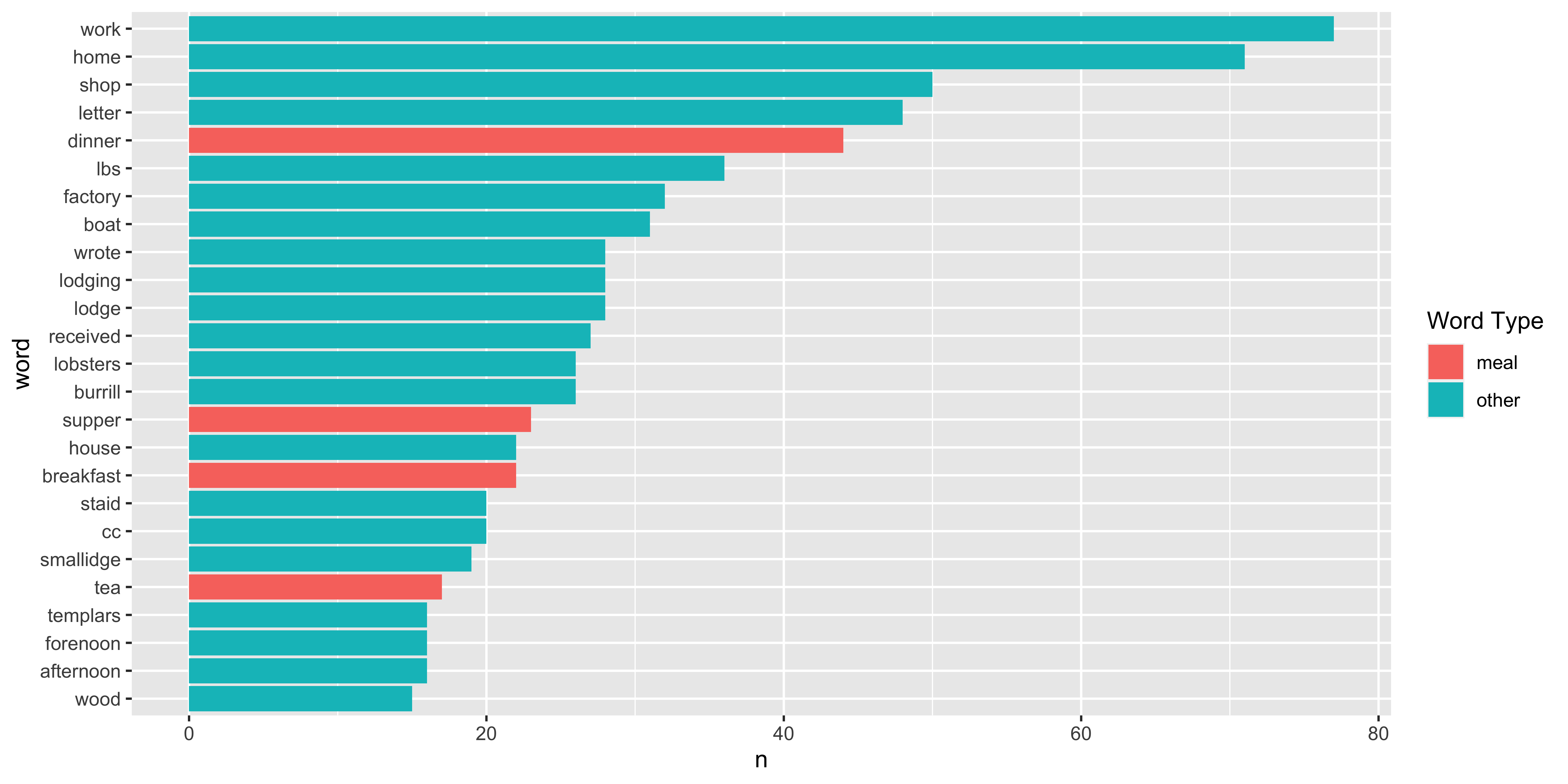
Journal 1: Boats, Meals, Goods 🍳 ⛵🦞 🪵

Journal 2: Wind and Weather ☁︎ NESW

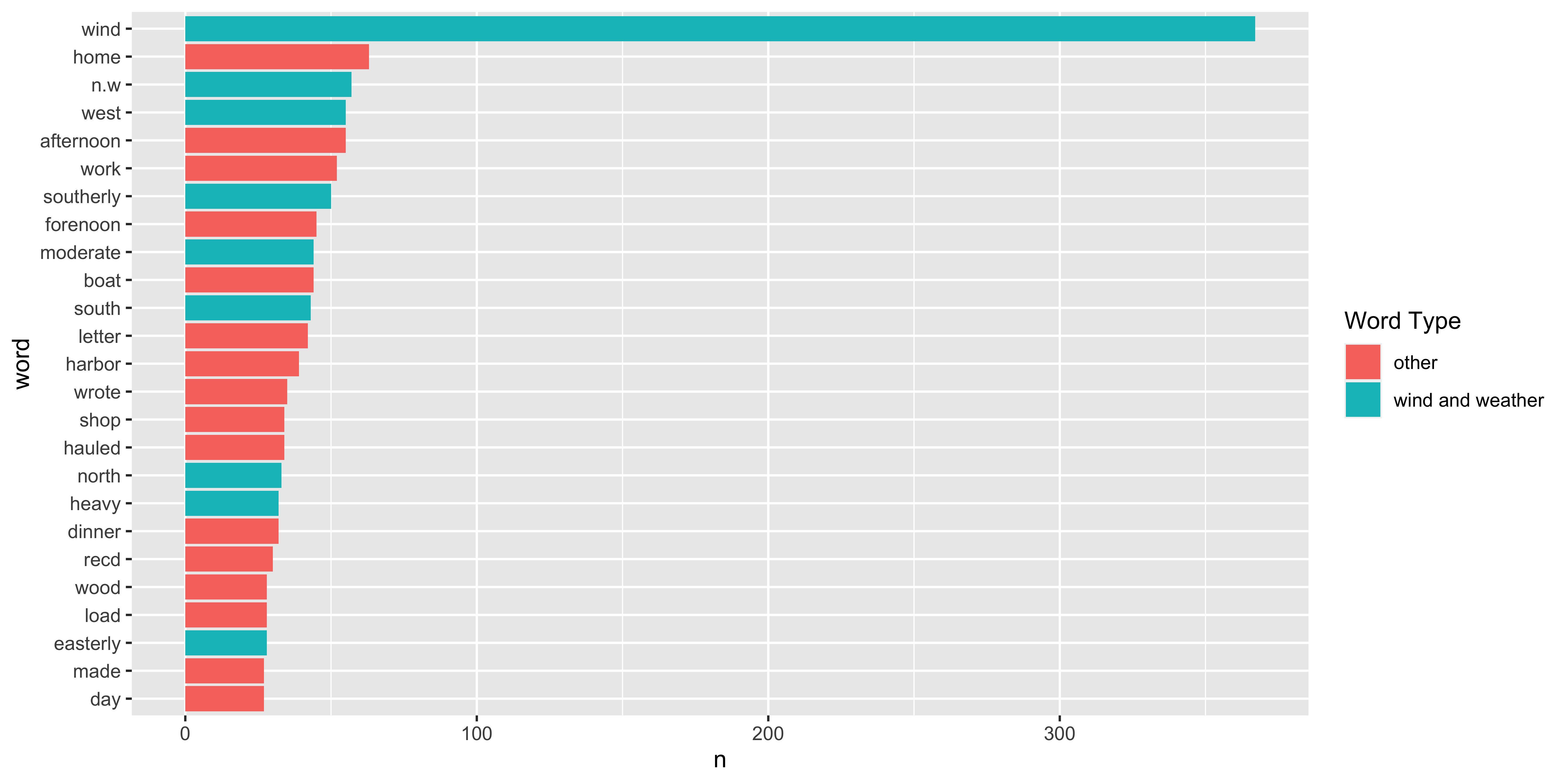
Your Turn: What were the most common words in Journal 3 and 4?

SENTIMENT ANALYSIS
😄😢😠

Sentiment lexicons

get_sentiments("afinn")
#> # A tibble: 2,477 × 2
#>    word       value
#>    <chr>      <dbl>
#>  1 abandon       -2
#>  2 abandoned     -2
#>  3 abandons      -2
#>  4 abducted      -2
#>  5 abduction     -2
#>  6 abductions    -2
#>  7 abhor         -3
#>  8 abhorred      -3
#>  9 abhorrent     -3
#> 10 abhors        -3
#> # ℹ 2,467 more rows

Sentiment lexicons

get_sentiments("bing")
#> # A tibble: 6,786 × 2
#>    word        sentiment
#>    <chr>       <chr>    
#>  1 2-faces     negative 
#>  2 abnormal    negative 
#>  3 abolish     negative 
#>  4 abominable  negative 
#>  5 abominably  negative 
#>  6 abominate   negative 
#>  7 abomination negative 
#>  8 abort       negative 
#>  9 aborted     negative 
#> 10 aborts      negative 
#> # ℹ 6,776 more rows

Sentiment lexicons

get_sentiments("nrc")
#> # A tibble: 13,872 × 2
#>    word        sentiment
#>    <chr>       <chr>    
#>  1 abacus      trust    
#>  2 abandon     fear     
#>  3 abandon     negative 
#>  4 abandon     sadness  
#>  5 abandoned   anger    
#>  6 abandoned   fear     
#>  7 abandoned   negative 
#>  8 abandoned   sadness  
#>  9 abandonment anger    
#> 10 abandonment fear     
#> # ℹ 13,862 more rows

Sentiment lexicons

get_sentiments("loughran")
#> # A tibble: 4,150 × 2
#>    word         sentiment
#>    <chr>        <chr>    
#>  1 abandon      negative 
#>  2 abandoned    negative 
#>  3 abandoning   negative 
#>  4 abandonment  negative 
#>  5 abandonments negative 
#>  6 abandons     negative 
#>  7 abdicated    negative 
#>  8 abdicates    negative 
#>  9 abdicating   negative 
#> 10 abdication   negative 
#> # ℹ 4,140 more rows

Implementing sentiment analysis

tidy_book %>%
    inner_join(get_sentiments("bing")) %>% 
    count(sentiment, sort = TRUE)
#> # A tibble: 0 × 2
#> # ℹ 2 variables: sentiment <chr>, n <int>

Jane wants to know…

What kind of join is appropriate for sentiment analysis?

• anti_join()
• full_join()
• outer_join()
• inner_join()

Implementing sentiment analysis

What do you predict will happen if we run the following code? 🤔

tidy_book %>%
    inner_join(get_sentiments("bing")) %>%            
    count(sentiment, word, sort = TRUE) 

Implementing sentiment analysis

What do you predict will happen if we run the following code? 🤔

tidy_book %>%
    inner_join(get_sentiments("bing")) %>%            
    count(sentiment, word, sort = TRUE)   
#> # A tibble: 0 × 3
#> # ℹ 3 variables: sentiment <chr>, word <chr>, n <int>

Implementing sentiment analysis

tidy_book %>%
    inner_join(get_sentiments("bing")) %>%
    count(sentiment, word, sort = TRUE) %>%
    group_by(sentiment) %>%
    slice_max(n, n = 10) %>%
    ungroup() %>%
    ggplot(aes(n, fct_reorder(word, n), fill = sentiment)) +
    geom_col() +
    facet_wrap(~sentiment, scales = "free") 

Was Freeland Sentimental?

Implementing sentiment analysis

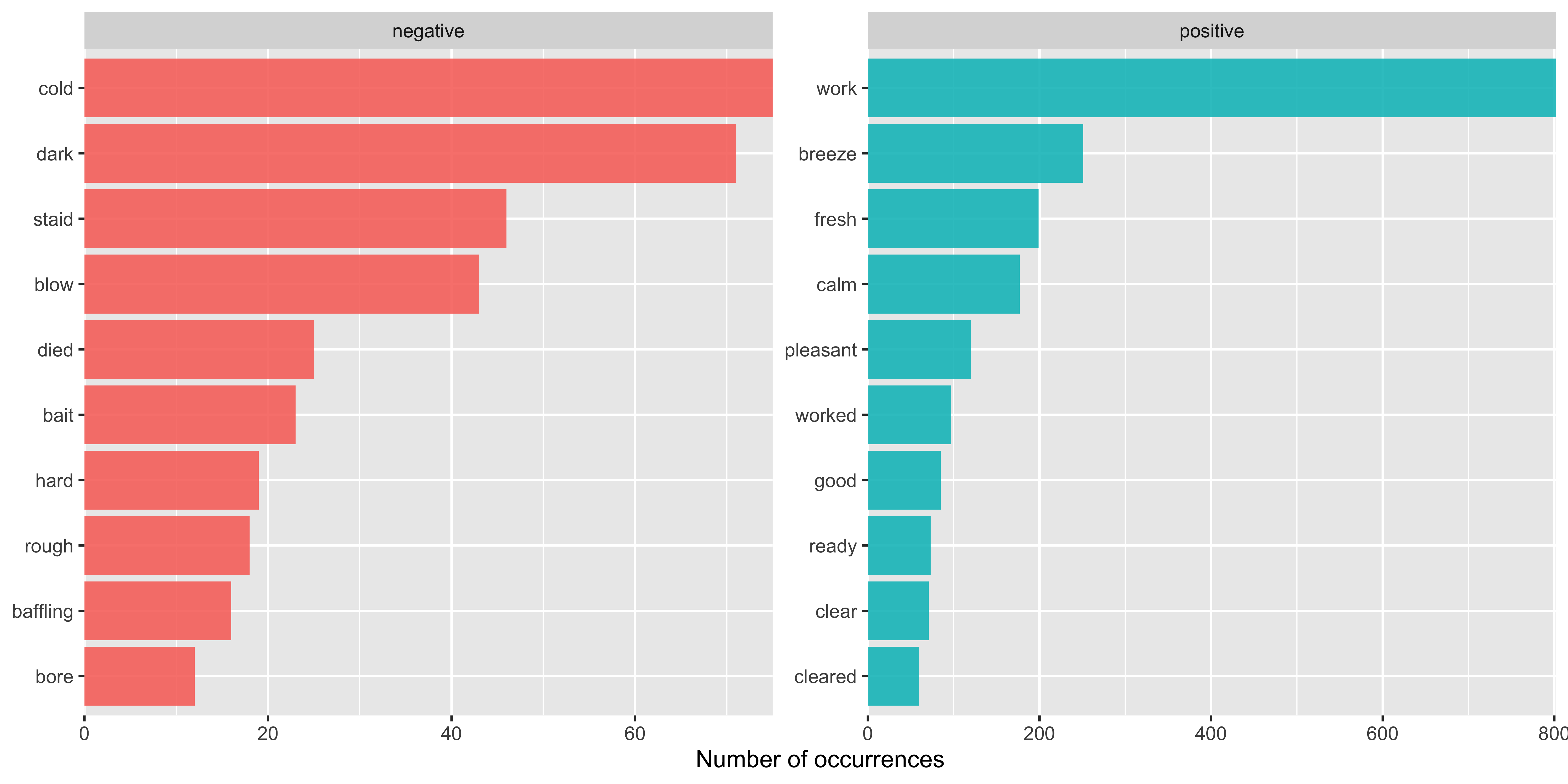
tidy_journal %>%
    inner_join(get_sentiments("bing")) %>%            
    count(sentiment, word, sort = TRUE)   
#> # A tibble: 198 × 3
#>    sentiment word         n
#>    <chr>     <chr>    <int>
#>  1 positive  work       802
#>  2 positive  breeze     251
#>  3 positive  fresh      199
#>  4 positive  calm       177
#>  5 positive  pleasant   120
#>  6 positive  worked      97
#>  7 positive  good        85
#>  8 negative  cold        75
#>  9 positive  ready       73
#> 10 negative  dark        71
#> # ℹ 188 more rows

Implementing sentiment analysis

tidy_journal %>%
    inner_join(get_sentiments("bing")) %>%
    count(sentiment, word, sort = TRUE) %>%
    group_by(sentiment) %>%
    slice_max(n, n = 10) %>%
    ungroup() %>%
    ggplot(aes(n, fct_reorder(word, n), fill = sentiment)) +
    geom_col() +
    facet_wrap(vars(sentiment), scales = "free") 

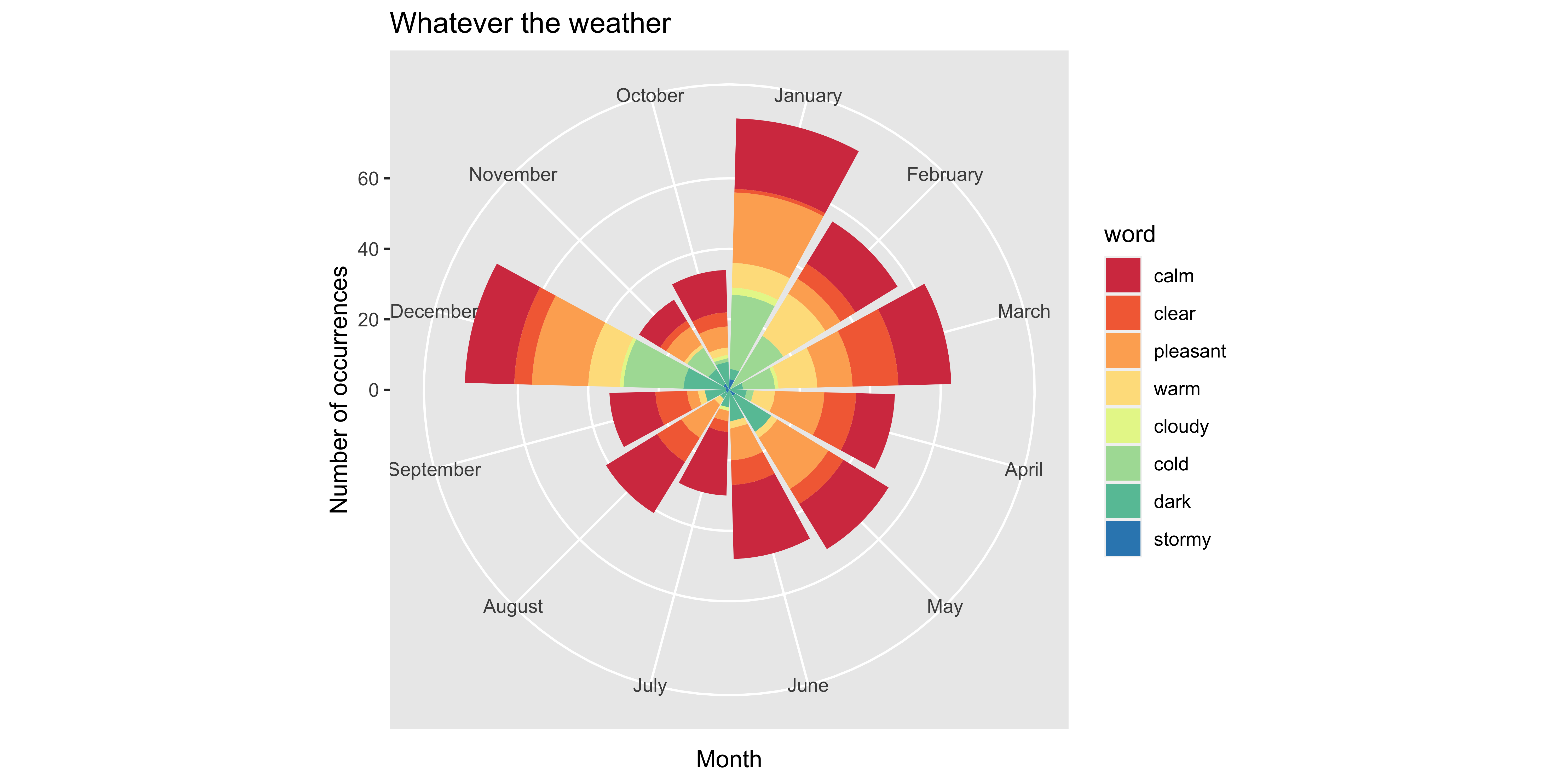
What was the weather like?

More insight from bigrams!

(tidy_ngram <- journals %>%
    mutate(journal_entry = str_replace_all(journal_entry, "south west", "southwest")) %>%
    mutate(journal_entry = str_replace_all(journal_entry, "north west", "northwest")) %>%
    mutate(journal_entry = str_replace_all(journal_entry, "south east", "southeast")) %>%
    mutate(journal_entry = str_replace_all(journal_entry, "north east", "northeast")) %>%
    unnest_tokens(bigram, journal_entry, token = "ngrams", n = 2) %>% 
    drop_na(bigram) %>%
    select(journal, bigram, date_mdy))
#> # A tibble: 61,170 × 3
#>    journal bigram       date_mdy  
#>      <dbl> <chr>        <chr>     
#>  1       1 was married  12/23/1871
#>  2       1 married at   12/23/1871
#>  3       1 at home      12/23/1871
#>  4       1 home in      12/23/1871
#>  5       1 in evening   12/23/1871
#>  6       1 evening by   12/23/1871
#>  7       1 by william   12/23/1871
#>  8       1 william rand 12/23/1871
#>  9       1 rand esqr    12/23/1871
#> 10       1 went to      12/24/1871
#> # ℹ 61,160 more rows

N-grams… and beyond! 🚀

tidy_ngram %>%
    count(bigram, sort = TRUE)
#> # A tibble: 19,375 × 2
#>    bigram             n
#>    <chr>          <int>
#>  1 the wind        2760
#>  2 in the           736
#>  3 wind north       572
#>  4 went to          558
#>  5 wind southerly   543
#>  6 all day          483
#>  7 north west       402
#>  8 wind south       378
#>  9 the afternoon    292
#> 10 work in          273
#> # ℹ 19,365 more rows

Jane wants to know…

Can we use an anti_join() now to remove stop words?

• Yes! ✅
• No ☹️

N-grams… and beyond! 🚀

bigram_counts <- tidy_ngram %>%
    separate(bigram, c("word1", "word2"), sep = " ") %>%
    filter(!word1 %in% stop_words$word,
           !word2 %in% stop_words$word) %>%
    count(word1, word2, sort = TRUE)

So many wind directions…! 🚀

bigram_counts
#> # A tibble: 7,230 × 3
#>    word1 word2           n
#>    <chr> <chr>       <int>
#>  1 wind  north         572
#>  2 wind  southerly     543
#>  3 north west          402
#>  4 wind  south         378
#>  5 south west          271
#>  6 wrote letter        263
#>  7 wind  easterly      243
#>  8 west  thermometer   186
#>  9 wind  westerly      182
#> 10 fresh breeze        175
#> # ℹ 7,220 more rows

Let’s tidy these up

bigram_counts <- tidy_ngram %>%
    separate(bigram, c("word1", "word2"), sep = " ") %>%
    filter(!word1 %in% stop_words$word,
           !word2 %in% stop_words$word) %>%
    mutate(word1 = case_when(word1 == "easterly" ~ "east",
                             word1 == "southerly" ~ "south",
                             word1 == "n.w" ~ "northwest",
                             word1 == "northerly" ~ "north",
                             word1 == "westerly" ~ "west",
           TRUE ~ word1)) %>%
    mutate(word2 = case_when(word2 == "easterly" ~ "east",
                             word2 == "southerly" ~ "south",
                             word2 == "n.w" ~ "northwest",
                             word2 == "northerly" ~ "north",
                             word2 == "westerly" ~ "west",
           TRUE ~ word2)) %>%
    count(word1, word2, sort = TRUE)

Removing wind

bigram_counts %>%
    filter(word1 != "wind" & word1 != "north" & word1 != "south")
#> # A tibble: 6,937 × 3
#>    word1 word2           n
#>    <chr> <chr>       <int>
#>  1 wrote letter        263
#>  2 west  thermometer   226
#>  3 fresh breeze        175
#>  4 west  gouldsboro    116
#>  5 east  thermometer    97
#>  6 reed  letter         96
#>  7 recd  letter         85
#>  8 heavy rain           82
#>  9 wm    guptill        67
#> 10 wrote letters        66
#> # ℹ 6,927 more rows

Thanks!

@juliasilge

@juliasilge

youtube.com/juliasilge

juliasilge.com

tidytextmining.com