Mining Historical Texts

USING TIDY DATA PRINCIPLES

By Laurie Baker

Acknowledgements

Slide Structure, Content, and Design adapted from Julia Silge

Let’s install some packages

install.packages(c("tidyverse", # data wrangling
                   "tidytext", # text analysis
                   "stopwords", # stop words
                   "lubridate", # dates
                   "readxl")) # reading data

The Journals (1870-1906)

What do we mean by tidy text?

journal_text <- c("Was married at home in evening by William Rand Esqr.",
          "Went to meeting.",
          "Shooting match all day in the evening to Christmas Tree at the Hall.",
          "About home at work fobbing.",
          "Work about home.",
          "To work in shop.",
          "To work in shop.",
          "Went to meeting.")

journal_text
#> [1] "Was married at home in evening by William Rand Esqr."                
#> [2] "Went to meeting."                                                    
#> [3] "Shooting match all day in the evening to Christmas Tree at the Hall."
#> [4] "About home at work fobbing."                                         
#> [5] "Work about home."                                                    
#> [6] "To work in shop."                                                    
#> [7] "To work in shop."                                                    
#> [8] "Went to meeting."

What do we mean by tidy text?

library(tidyverse)

journal_df <- tibble(line = 1:8, text = journal_text)

journal_df
#> # A tibble: 8 × 2
#>    line text                                                                
#>   <int> <chr>                                                               
#> 1     1 Was married at home in evening by William Rand Esqr.                
#> 2     2 Went to meeting.                                                    
#> 3     3 Shooting match all day in the evening to Christmas Tree at the Hall.
#> 4     4 About home at work fobbing.                                         
#> 5     5 Work about home.                                                    
#> 6     6 To work in shop.                                                    
#> 7     7 To work in shop.                                                    
#> 8     8 Went to meeting.

What do we mean by tidy text?

library(tidytext)

journal_df %>%
    unnest_tokens(word, text)
#> # A tibble: 45 × 2
#>     line word   
#>    <int> <chr>  
#>  1     1 was    
#>  2     1 married
#>  3     1 at     
#>  4     1 home   
#>  5     1 in     
#>  6     1 evening
#>  7     1 by     
#>  8     1 william
#>  9     1 rand   
#> 10     1 esqr   
#> # ℹ 35 more rows

Freeland wants to know…

A tidy text dataset typically has

more
fewer

rows than the original, non-tidy text dataset.

9 journals (1871-1880) transcribed


journals <- read_csv(file = "data/journals.csv")

journals %>%
    distinct(journal)
#> # A tibble: 9 × 1
#>   journal
#>     <dbl>
#> 1       1
#> 2       2
#> 3       3
#> 4       4
#> 5       5
#> 6       6
#> 7       7
#> 8       8
#> 9       9

Journal Date, Text, and Location

journals %>%
    select(date_mdy, journal_entry, location)
#> # A tibble: 3,951 × 3
#>    date_mdy   journal_entry                                             location
#>    <chr>      <chr>                                                     <chr>   
#>  1 12/23/1871 Was married at home in evening by William Rand Esqr.      Winter …
#>  2 12/24/1871 Went to meeting.                                          <NA>    
#>  3 12/25/1871 Shooting match all day in the evening to Christmas tree … Winter …
#>  4 12/26/1871 About home at work fobbing.                               Winter …
#>  5 12/27/1871 Work about home reed letter from N. H. Higgins Ins agt.   Winter …
#>  6 12/28/1871 Work about home.                                          Winter …
#>  7 12/29/1871 To work in shop.                                          Winter …
#>  8 12/30/1871 To work in shop.                                          Winter …
#>  9 12/31/1871 Went to meeting.                                          <NA>    
#> 10 1/1/1872   Work in shop.                                             Winter …
#> # ℹ 3,941 more rows

Creating date variables using `lubridate`

Recall: What functions can we use to extract the year and month?

library(lubridate)
journals <- journals %>%
    select(date_mdy, journal_entry, journal, location) %>%
    mutate(date_mdy = mdy(date_mdy),
           year = _____(date_mdy),
           month = _____(date_mdy))

Hint: Check the lubridate cheatsheet

Creating date variables using `lubridate`

library(lubridate)
(journals <- journals %>%
    select(date_mdy, journal_entry, journal, location) %>%
    mutate(date_mdy = mdy(date_mdy),
           year = year(date_mdy),
           month = month(date_mdy)))
#> # A tibble: 3,951 × 6
#>    date_mdy   journal_entry                         journal location  year month
#>    <date>     <chr>                                   <dbl> <chr>    <dbl> <dbl>
#>  1 1871-12-23 Was married at home in evening by Wi…       1 Winter …  1871    12
#>  2 1871-12-24 Went to meeting.                            1 <NA>      1871    12
#>  3 1871-12-25 Shooting match all day in the evenin…       1 Winter …  1871    12
#>  4 1871-12-26 About home at work fobbing.                 1 Winter …  1871    12
#>  5 1871-12-27 Work about home reed letter from N. …       1 Winter …  1871    12
#>  6 1871-12-28 Work about home.                            1 Winter …  1871    12
#>  7 1871-12-29 To work in shop.                            1 Winter …  1871    12
#>  8 1871-12-30 To work in shop.                            1 Winter …  1871    12
#>  9 1871-12-31 Went to meeting.                            1 <NA>      1871    12
#> 10 1872-01-01 Work in shop.                               1 Winter …  1872     1
#> # ℹ 3,941 more rows

Making our text data tidy

(tidy_journal <- journals %>%
    unnest_tokens(word, journal_entry))
#> # A tibble: 65,118 × 6
#>    date_mdy   journal location       year month word   
#>    <date>       <dbl> <chr>         <dbl> <dbl> <chr>  
#>  1 1871-12-23       1 Winter Harbor  1871    12 was    
#>  2 1871-12-23       1 Winter Harbor  1871    12 married
#>  3 1871-12-23       1 Winter Harbor  1871    12 at     
#>  4 1871-12-23       1 Winter Harbor  1871    12 home   
#>  5 1871-12-23       1 Winter Harbor  1871    12 in     
#>  6 1871-12-23       1 Winter Harbor  1871    12 evening
#>  7 1871-12-23       1 Winter Harbor  1871    12 by     
#>  8 1871-12-23       1 Winter Harbor  1871    12 william
#>  9 1871-12-23       1 Winter Harbor  1871    12 rand   
#> 10 1871-12-23       1 Winter Harbor  1871    12 esqr   
#> # ℹ 65,108 more rows

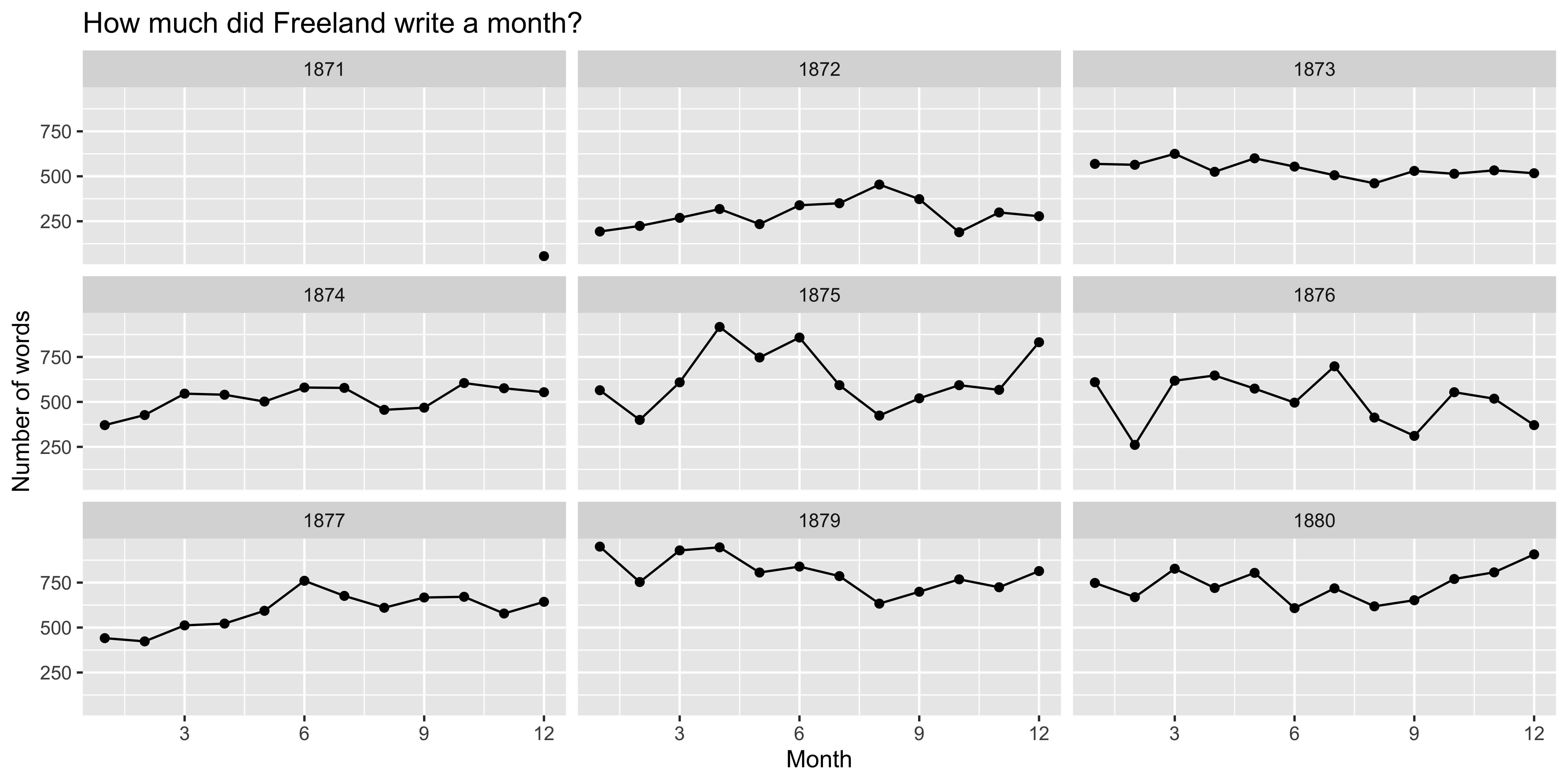
How much did Freeland write?

(monthly_word_count <- tidy_journal %>%
  group_by(month, year) %>%
  filter(is.na(year) == FALSE) %>%
  summarize(nwords = n()))
#> # A tibble: 97 × 3
#> # Groups:   month [12]
#>    month  year nwords
#>    <dbl> <dbl>  <int>
#>  1     1  1872    193
#>  2     1  1873    569
#>  3     1  1874    371
#>  4     1  1875    565
#>  5     1  1876    610
#>  6     1  1877    441
#>  7     1  1879    950
#>  8     1  1880    748
#>  9     2  1872    224
#> 10     2  1873    564
#> # ℹ 87 more rows

Plotting monthly word count through time

What plot do you expect to see?

monthly_word_count %>%
  ggplot(aes(x = month, y = nwords, group = year)) +
  geom_line() +
  geom_point() +
  facet_wrap(~year) +
  labs(title = "How much did Freeland write a month?",
       y = "Number of words",
       x = "Month") +
  scale_x_continuous(breaks = c(0, 3, 6, 9, 12))

How much did Freeland write?

What are the most common words?

What do you predict will happen if we run the following code? 🤔

tidy_journal %>%
    count(word, sort = TRUE)

What are the most common words?

What do you predict will happen if we run the following code? 🤔

tidy_journal %>%
    count(word, sort = TRUE)
#> # A tibble: 4,105 × 2
#>    word            n
#>    <chr>       <int>
#>  1 the          5116
#>  2 wind         3052
#>  3 and          2301
#>  4 in           2181
#>  5 to           1959
#>  6 at           1422
#>  7 thermometer  1071
#>  8 of            948
#>  9 west          933
#> 10 went          909
#> # ℹ 4,095 more rows

Stop words

get_stopwords()
#> # A tibble: 175 × 2
#>    word      lexicon 
#>    <chr>     <chr>   
#>  1 i         snowball
#>  2 me        snowball
#>  3 my        snowball
#>  4 myself    snowball
#>  5 we        snowball
#>  6 our       snowball
#>  7 ours      snowball
#>  8 ourselves snowball
#>  9 you       snowball
#> 10 your      snowball
#> # ℹ 165 more rows

Stop words

get_stopwords(language = "es")
#> # A tibble: 308 × 2
#>    word  lexicon 
#>    <chr> <chr>   
#>  1 de    snowball
#>  2 la    snowball
#>  3 que   snowball
#>  4 el    snowball
#>  5 en    snowball
#>  6 y     snowball
#>  7 a     snowball
#>  8 los   snowball
#>  9 del   snowball
#> 10 se    snowball
#> # ℹ 298 more rows

Stop words

get_stopwords(language = "de")
#> # A tibble: 231 × 2
#>    word  lexicon 
#>    <chr> <chr>   
#>  1 aber  snowball
#>  2 alle  snowball
#>  3 allem snowball
#>  4 allen snowball
#>  5 aller snowball
#>  6 alles snowball
#>  7 als   snowball
#>  8 also  snowball
#>  9 am    snowball
#> 10 an    snowball
#> # ℹ 221 more rows

Stop words

get_stopwords(source = "smart")
#> # A tibble: 571 × 2
#>    word        lexicon
#>    <chr>       <chr>  
#>  1 a           smart  
#>  2 a's         smart  
#>  3 able        smart  
#>  4 about       smart  
#>  5 above       smart  
#>  6 according   smart  
#>  7 accordingly smart  
#>  8 across      smart  
#>  9 actually    smart  
#> 10 after       smart  
#> # ℹ 561 more rows

What are the most common words?

U N S C R A M B L E

anti_join(get_stopwords(source = “smart”)) %>%

tidy_journal %>%

count(word, sort = TRUE) %>%

geom_col() +

slice_max(n, n = 20) %>%

ggplot(aes(n, fct_reorder(word, n))) +

What are the most common words?

tidy_journal %>%
    anti_join(get_stopwords(source = "smart")) %>%
    count(word, sort = TRUE) %>%
    slice_max(n, n = 20) %>%
    ggplot(aes(n, fct_reorder(word, n))) +  
    geom_col()

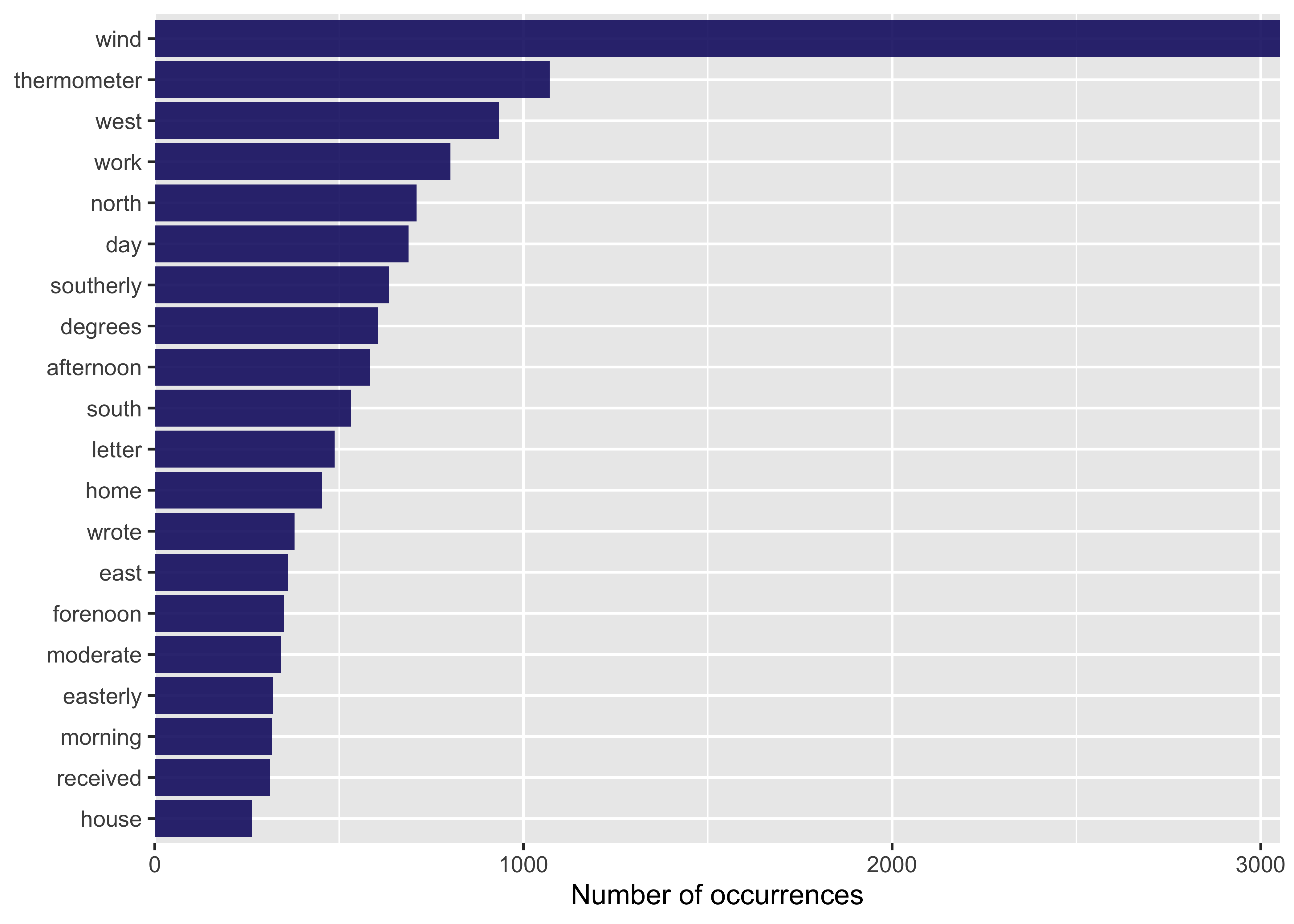
Journal 1: Boats, Meals, Goods 🍳 ⛵🦞 🪵

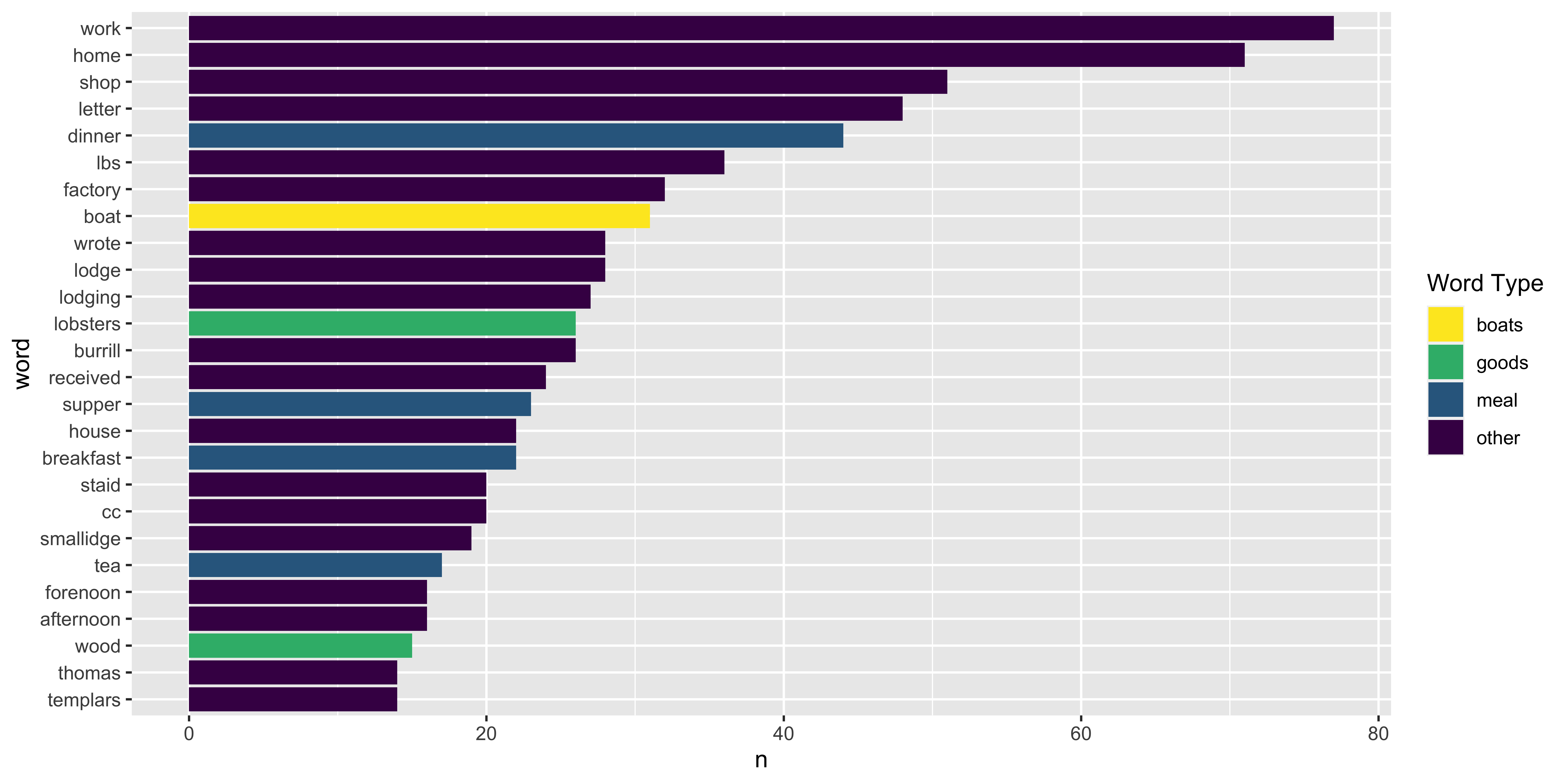
Journal 2: Wind and Weather︎ NESW

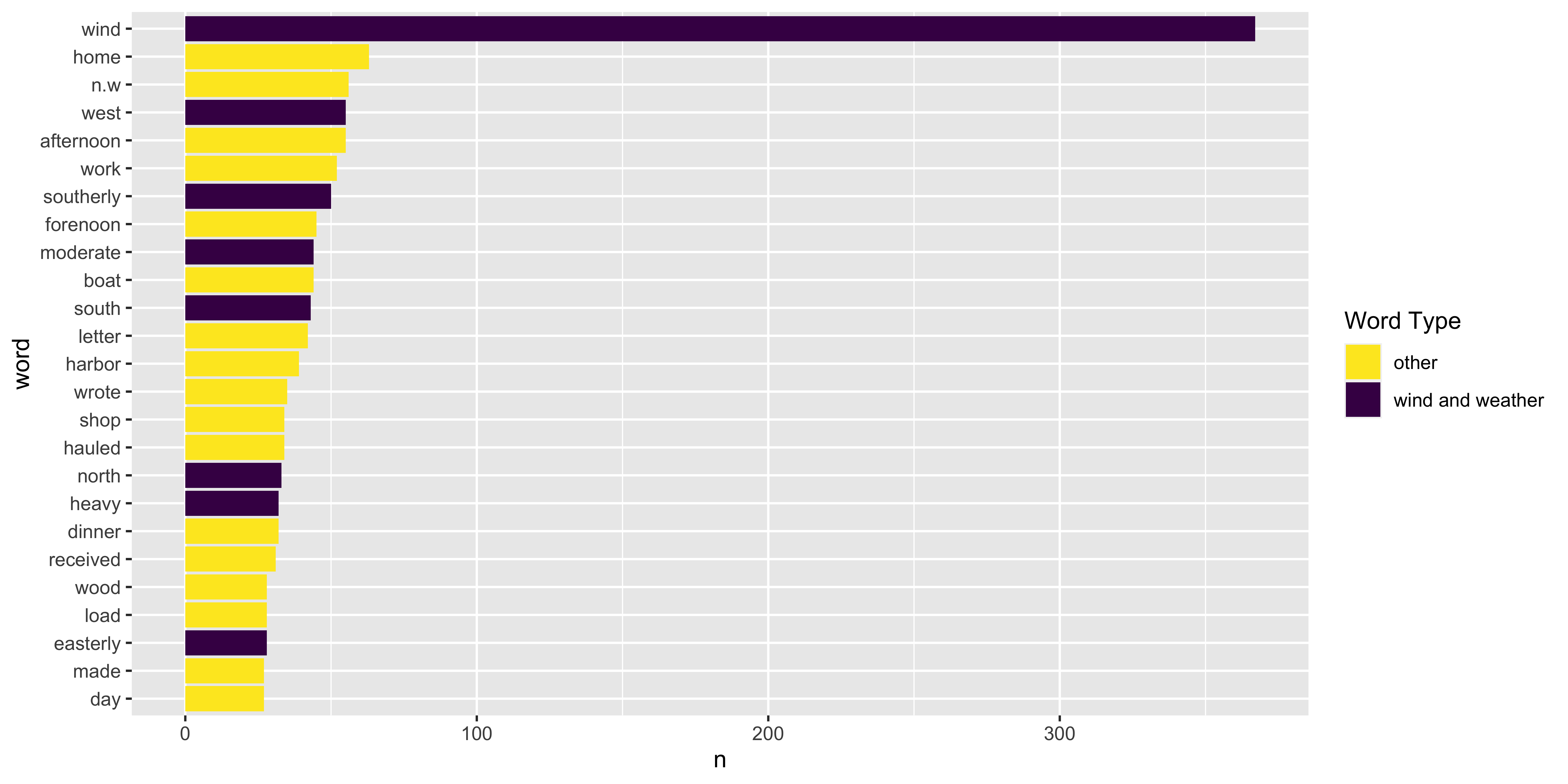
Comparing multiple journals

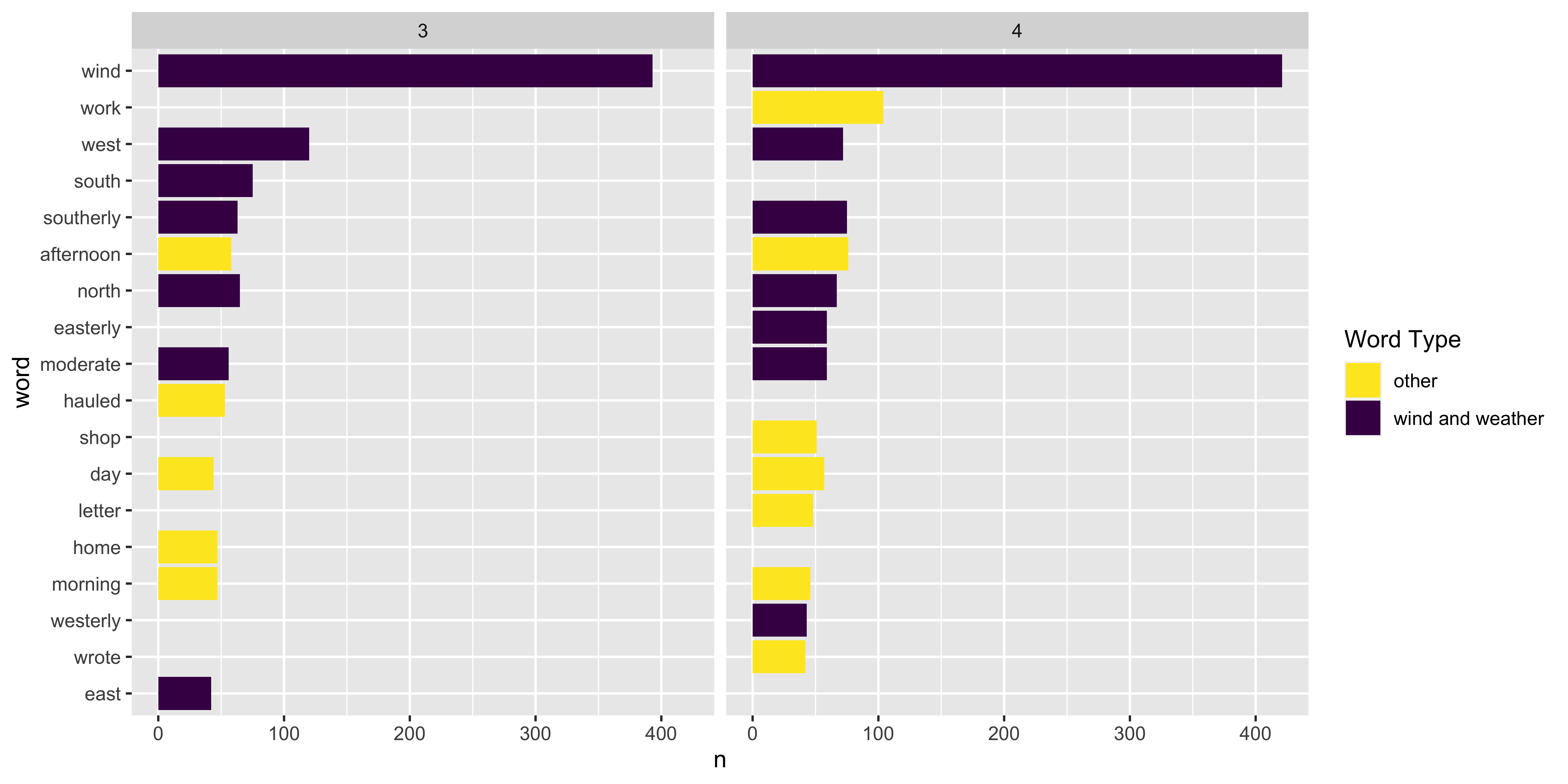
Your Turn: What were the most common words in Journal 5 and 6?

tidy_journal %>%
    anti_join(get_stopwords(source = "smart")) %>%
    filter(journal %in% c(____, ____)) %>%
    count(word, sort = TRUE) %>%
    slice_max(n, n = 25) %>%
    ggplot(aes(n, fct_reorder(word, n))) +  
    geom_col(aes(fill = color)) +
    labs(fill = "Word Type", y = "word") +
    scale_fill_viridis_d(direction = -1)

Your Turn: What were the most common words in your journal period?

tidy_journal %>%
    anti_join(get_stopwords(source = "smart")) %>%
    filter(year _______,
           month %in% c(_________)) %>%
    count(word, sort = TRUE) %>%
    slice_max(n, n = 25) %>%
    ggplot(aes(n, fct_reorder(word, n))) +  
    geom_col(aes(fill = color)) +
    labs(fill = "Word Type", y = "word") +
    scale_fill_viridis_d(direction = -1)

Looking at word trends through space

tidy_journal %>%
    anti_join(get_stopwords(source = "smart")) %>%
    filter(str_detect(location, pattern = "Matinicus")) %>%
    count(word, sort = TRUE) %>%
    filter(word != "home") %>%
    slice_max(n, n = 10, with_ties = FALSE) %>%
    ggplot(aes(n, fct_reorder(word, n))) +  
    geom_col() +
    labs(fill = "Word Type", y = "word", title = "Matinicus") +
    scale_fill_viridis_d(direction = -1)

Looking at word trends through space

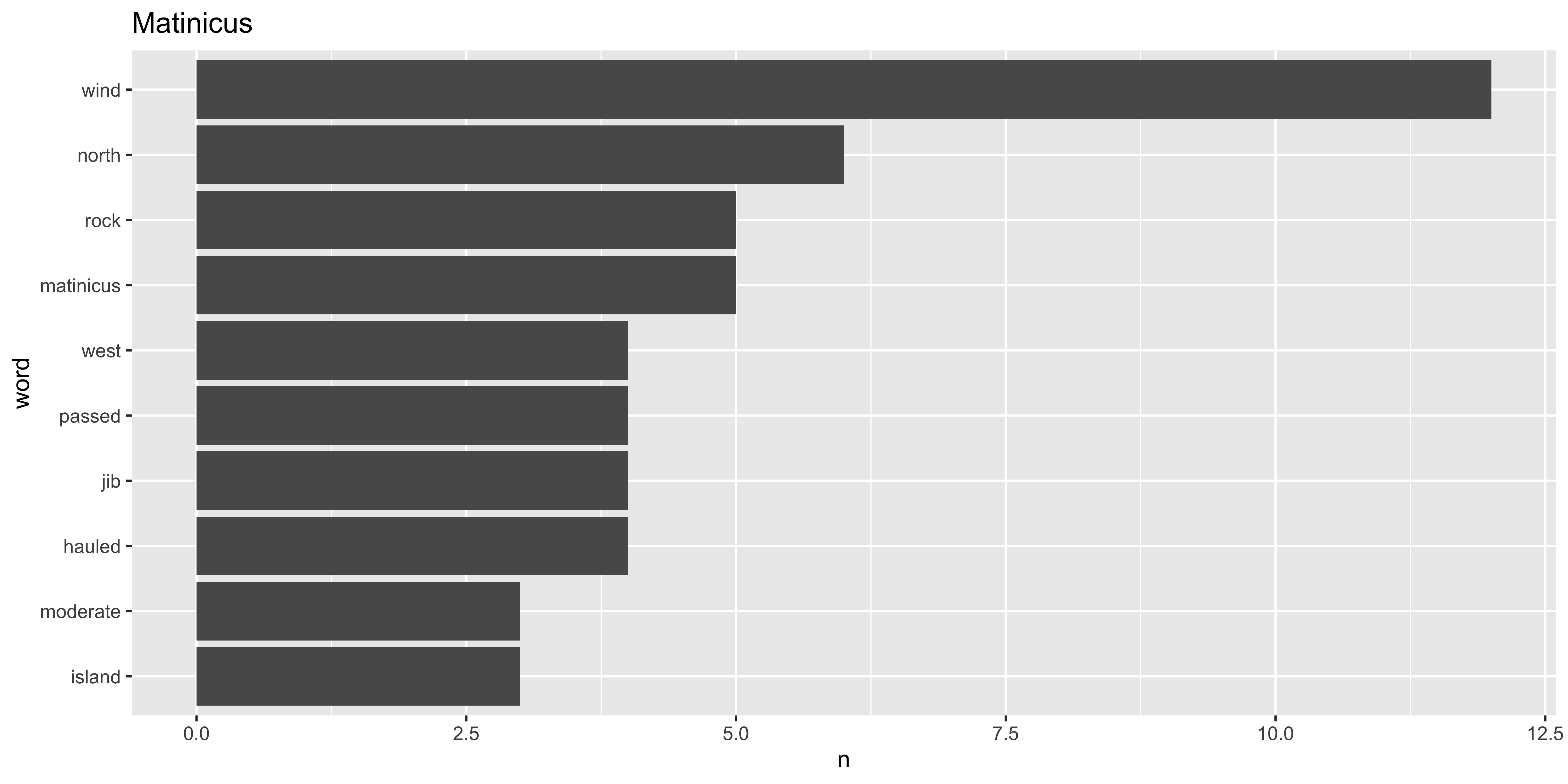
Your Turn: Looking at word trends through space

tidy_journal %>%
    anti_join(get_stopwords(source = "smart")) %>%
    filter(str_detect(location, "__________")) %>%
    count(word, sort = TRUE) %>%
    slice_max(n, n = 10, with_ties = FALSE) %>%
    ggplot(aes(n, fct_reorder(word, n))) +  
    geom_col() +
    labs(fill = "Word Type", y = "word", title = "_______") +
    scale_fill_viridis_d(direction = -1)

We can also look for specific things

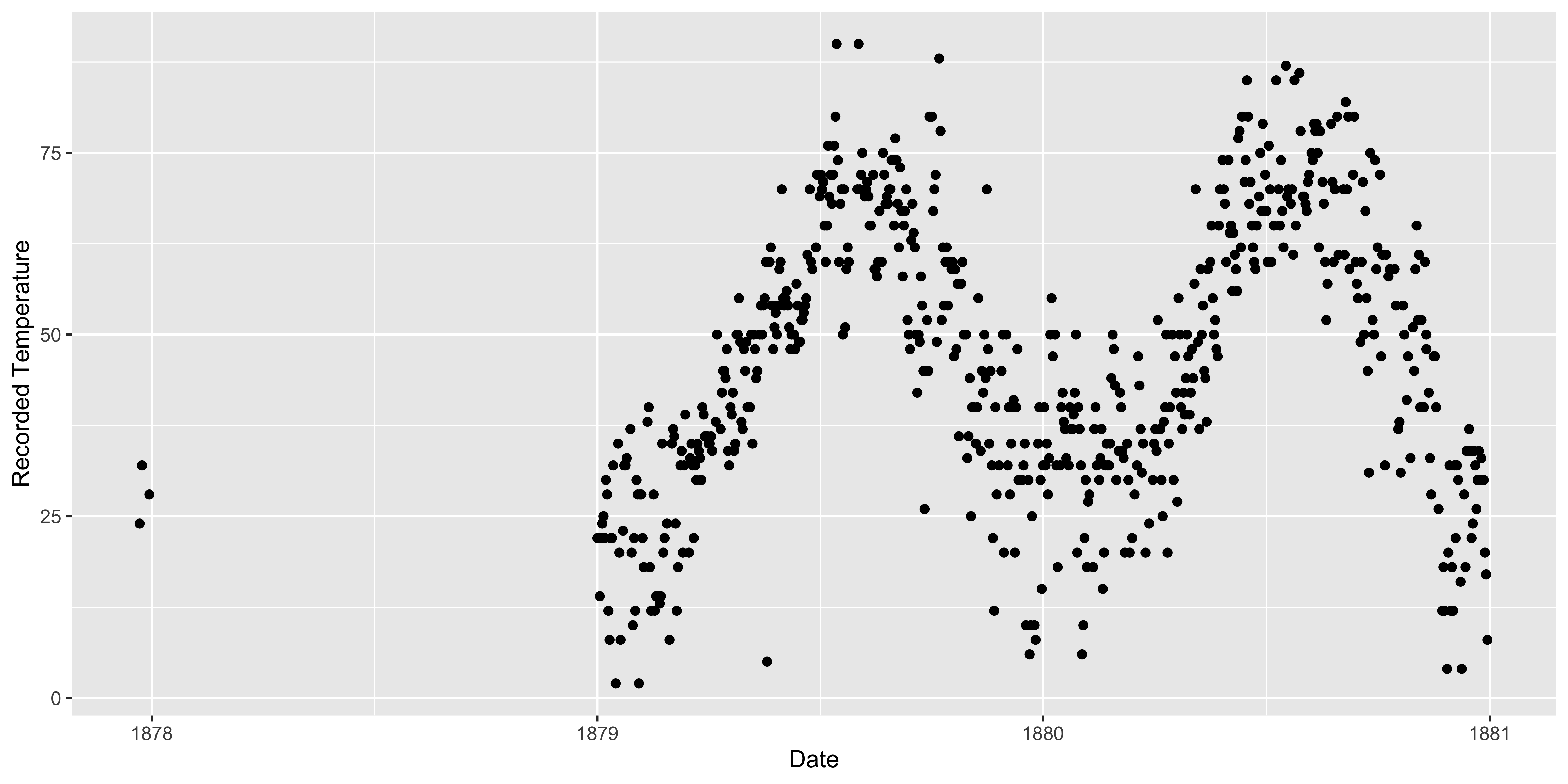
Extracting thermometer readings

journals %>%
  filter(str_detect(string = journal_entry, pattern = "Thermometer | thermometer")) %>% # filter rows for mentions of word thermometer
  mutate(temp = as.numeric(str_extract(journal_entry, pattern = '(?<=thermometer |Thermometer )\\d+'))) %>% # extract digits following the word thermometer in a sentence.
  ggplot(aes(x = date_mdy, y = as.numeric(temp))) +
  geom_point() +
  labs(x = "Date", y = "Recorded Temperature")

Looking for Schooners

journals %>%
    filter(str_detect(journal_entry, pattern = "Schr|schr|schooner")) %>%
    select(date_mdy, journal_entry) %>%
    DT::datatable()

Extracting names of schooners

journals %>%
    filter(str_detect(journal_entry, pattern = "Schr|schr|schooner")) %>%
    mutate(schooners = str_extract(journal_entry, pattern = "\\b(Schr|Schr.|schr|schr.)(\\b\\s*([A-Z]\\w+|[A-Z]\\.\\w+\\.\\w+|[A-Z]\\. \\w+\\. \\w+)){0,4}")) %>%
    distinct(schooners)
#> # A tibble: 38 × 1
#>    schooners                         
#>    <chr>                             
#>  1 Schr A. G. Brooks                 
#>  2 schr Fremont Capt Elisher Bickford
#>  3 Schr Sea Flower                   
#>  4 schr Roamer                       
#>  5 schr Virgin                       
#>  6 schr Virgins                      
#>  7 Schr Roamer                       
#>  8 Schr Neptune                      
#>  9 Schr Banner                       
#> 10 Schr Signal                       
#> # ℹ 28 more rows

Recap

We can put each word on its own row using unnest_tokens
We can use anti_join to get rid of stop words
We can use filter and summarize to see how word use has changed over time and space
We can use str_detect to find patterns in our text
We can use regular expressions to extract more complicated patterns

Your Turn

What is something you are curious about in Freeland’s journals that you’d like to investigate? Be creative with the time period, place, and what you’re looking for.

journals %>%
    filter(str_detect(journal_entry, pattern = "What are you looking for?")) %>%
    select(date_mdy, journal_entry)

Thanks!

@LaurieLBaker

lauriebaker@rbind.io

Additional Slides

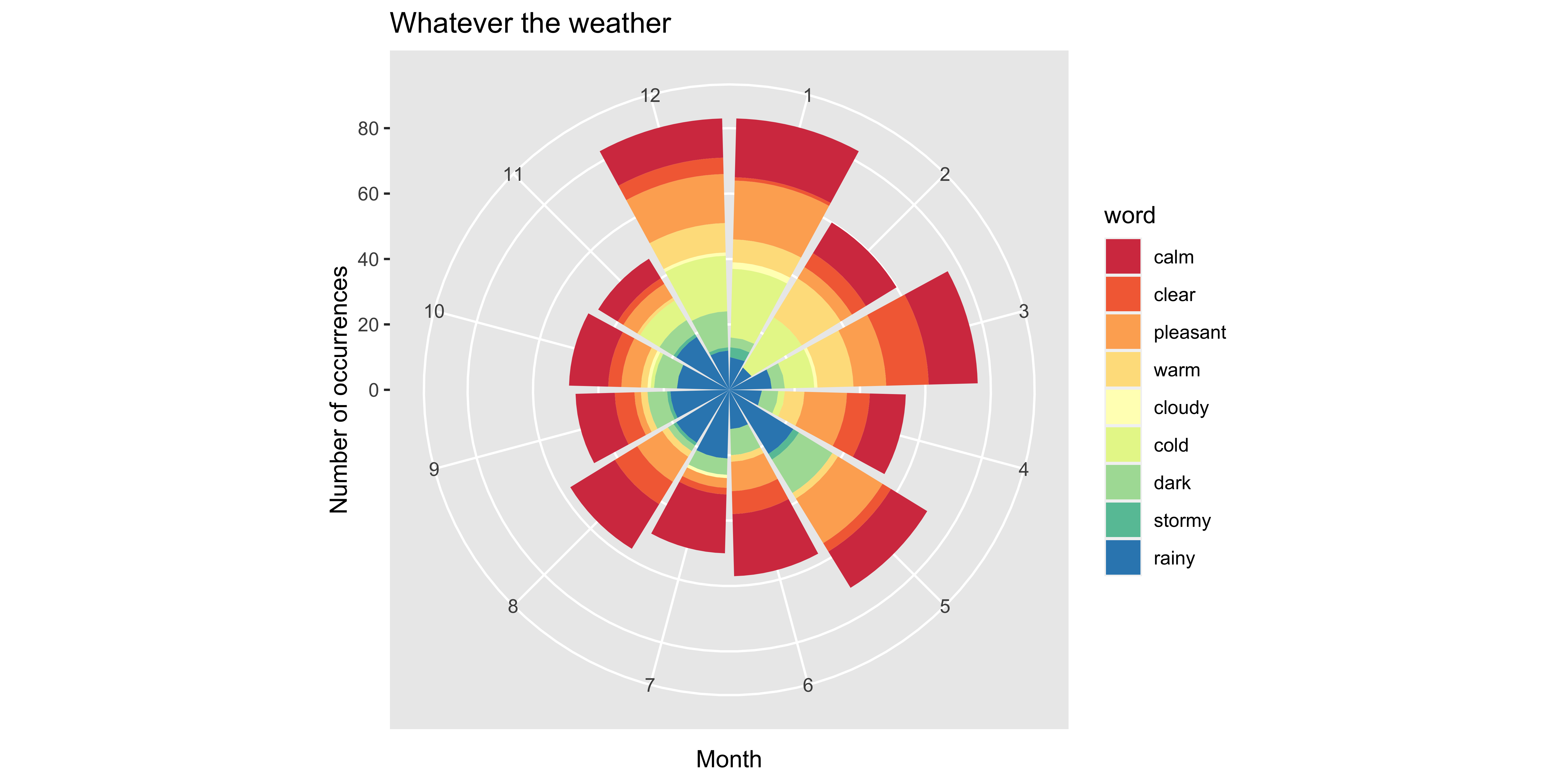
What was the weather like?

Mining Historical Texts

Acknowledgements

Let’s install some packages

The Journals (1870-1906)

What do we mean by tidy text?

What do we mean by tidy text?

What do we mean by tidy text?

Freeland wants to know…

9 journals (1871-1880) transcribed

Journal Date, Text, and Location

Creating date variables using lubridate

Creating date variables using lubridate

Making our text data tidy

How much did Freeland write?

Plotting monthly word count through time

How much did Freeland write?

What are the most common words?

What are the most common words?

Stop words

Stop words

Stop words

Stop words

What are the most common words?

What are the most common words?

Journal 1: Boats, Meals, Goods 🍳 ⛵🦞 🪵

Journal 2: Wind and Weather︎ NESW

Comparing multiple journals

Your Turn: What were the most common words in Journal 5 and 6?

Your Turn: What were the most common words in your journal period?

Looking at word trends through space

Looking at word trends through space

Your Turn: Looking at word trends through space

We can also look for specific things

Extracting thermometer readings

Extracting thermometer readings

Looking for Schooners

Extracting names of schooners

Recap

Your Turn

Thanks!

Additional Slides

What was the weather like?

Creating date variables using `lubridate`

Creating date variables using `lubridate`